การทำข้อมูลแผนที่และการแสดงผลขั้นสูง

เราจะเรียนรู้วิธี:

• การทำงานกับข้อมูลทางพื้นที่
• การสร้างแผนที่แบบโต้ตอบใน Shiny โดยใช้ Leaflet
• การใช้ Shiny events และ proxies

แผนที่แบบโต้ตอบ

• การทำแผนที่เป็นการแสดงผลข้อมูลที่ขึ้นอยู่กับ spatial data
• การทำแผนที่แบบดั้งเดิมพึ่งพา generalization และการตีความ (interpretation)
• การทำแผนที่แบบโต้ตอบลบข้อจำกัดหลาย ๆ อย่าง เช่น generalizationและขอบเขตแผนที่

Generalization in OpenStreetMap at different scales

สถานะ app ตอนนี้

• สรุปสั้น ๆ:
  • ในหัวข้อที่ 3 เราได้เพิ่ม tab แนะนำซึ่งมีข้อมูลพื้นฐานเกี่ยวกับapp
  • ในหัวข้อที่ 4 เราเพิ่ม tab ตารางที่ใช้ DT
  • ในหัวข้อที่ 5 เราเพิ่ม tab แบบจำลองโดยใช้การแสดงผลแบบต่าง ๆ

Full code for the current app state

library(shiny)
library(htmltools)
library(bs4Dash)
library(fresh)
library(waiter)
library(shinyWidgets)
library(Guerry)
library(sf)
library(tidyr)
library(dplyr)
library(RColorBrewer)
library(viridis)
library(leaflet)
library(plotly)
library(ggplot2)
library(GGally)
library(datawizard)
library(parameters)
library(performance)
library(modelsummary)

# 1 Data preparation ----

## Load & clean data ----
variable_names <- list(
  Crime_pers = "Crime against persons",  
  Crime_prop =  "Crime against property",  
  Literacy = "Literacy",  
  Donations = "Donations to the poor",  
  Infants = "Illegitimate births",  
  Suicides = "Suicides",  
  Wealth = "Tax / capita",  
  Commerce = "Commerce & Industry",  
  Clergy = "Clergy",  
  Crime_parents = "Crime against parents",  
  Infanticide = "Infanticides",  
  Donation_clergy = "Donations to the clergy",  
  Lottery = "Wager on Royal Lottery",  
  Desertion = "Military desertion",  
  Instruction = "Instruction",  
  Prostitutes = "Prostitutes",  
  Distance = "Distance to paris",  
  Area = "Area",  
  Pop1831 = "Population"
)

variable_desc <- list(
  Crime_pers = list(
    title = "Crime against persons",
    desc = as.character(p(tags$b("Crime against persons:"), "Population per crime against persons", hr(), helpText("Source: Table A2 in Guerry (1833). Compte général, 1825-1830"))),
    lgd = "Pop. per crime",
    unit = ""
  ),
  Crime_prop = list(
    title = "Crime against property",
    desc = as.character(p(tags$b("Crime against property:"), "Population per crime against property", hr(), helpText("Source: Compte général, 1825-1830"))),
    lgd = "Pop. per crime",
    unit = ""
  ),
  Literacy = list(
    title = "Literacy",
    desc = as.character(p(tags$b("Percent Read & Write:"), "Percent of military conscripts who can read and write", hr(), helpText("Source: Table A2 in Guerry (1833)"))),
    lgd = "Literacy",
    unit = " %"
  ),
  Donations = list(
    title = "Donations to the poor",
    desc = as.character(p(tags$b("Donations to the poor"), hr(), helpText("Source: Table A2 in Guerry (1833). Bulletin des lois"))),
    lgd = "Donations",
    unit = ""
  ),
  Infants = list(
    title = "Illegitimate births",
    desc = as.character(p(tags$b("Population per illegitimate birth"), hr(), helpText("Source: Table A2 in Guerry (1833). Bureau des Longitudes, 1817-1821"))),
    lgd = "Pop. per birth",
    unit = ""
  ),
  Suicides = list(
    title = "Suicides",
    desc = as.character(p(tags$b("Population per suicide"), hr(), helpText("Source: Table A2 in Guerry (1833). Compte général, 1827-1830"))),
    lgd = "Pop. per suicide",
    unit = ""
  ),
  Wealth = list(
    title = "Tax / capita",
    desc = as.character(p(tags$b("Per capita tax on personal property:"), "A ranked index based on taxes on personal and movable property per inhabitant", hr(), helpText("Source: Table A1 in Guerry (1833)"))),
    lgd = "Tax / capita",
    unit = ""
  ),
  Commerce = list(
    title = "Commerce & Industry",
    desc = as.character(p(tags$b("Commerce & Industry:"), "Commerce and Industry, measured by the rank of the number of patents / population", hr(), helpText("Source: Table A1 in Guerry (1833)"))),
    lgd = "Patents / capita",
    unit = ""
  ),
  Clergy = list(
    title = "Clergy",
    desc = as.character(p(tags$b("Distribution of clergy:"), "Distribution of clergy, measured by the rank of the number of Catholic priests in active service / population", hr(), helpText("Source: Table A1 in Guerry (1833). Almanach officiel du clergy, 1829"))),
    lgd = "Priests / capita",
    unit = ""
  ),
  Crime_parents = list(
    title = "Crime against parents",
    desc = as.character(p(tags$b("Crime against parents:"), "Crimes against parents, measured by the rank of the ratio of crimes against parents to all crimes \u2013 Average for the years 1825-1830", hr(), helpText("Source: Table A1 in Guerry (1833). Compte général"))),
    lgd = "Share of crimes",
    unit = " %"
  ),
  Infanticide = list(
    title = "Infanticides",
    desc = as.character(p(tags$b("Infanticides per capita:"), "Ranked ratio of number of infanticides to population \u2013 Average for the years 1825-1830", hr(), helpText("Source: Table A1 in Guerry (1833). Compte général"))),
    lgd = "Infanticides / capita",
    unit = ""
  ),
  Donation_clergy = list(
    title = "Donations to the clergy",
    desc = as.character(p(tags$b("Donations to the clergy:"), "Ranked ratios of the number of bequests and donations inter vivios to population \u2013 Average for the years 1815-1824", hr(), helpText("Source: Table A1 in Guerry (1833). Bull. des lois, ordunn. d’autorisation"))),
    lgd = "Donations / capita",
    unit = ""
  ),
  Lottery = list(
    title = "Wager on Royal Lottery",
    desc = as.character(p(tags$b("Per capita wager on Royal Lottery:"), "Ranked ratio of the proceeds bet on the royal lottery to population \u2013 Average for the years 1822-1826", hr(), helpText("Source: Table A1 in Guerry (1833). Compte rendu par le ministre des finances"))),
    lgd = "Wager / capita",
    unit = ""
  ),
  Desertion = list(
    title = "Military desertion",
    desc = as.character(p(tags$b("Military desertion:"), "Military disertion, ratio of the number of young soldiers accused of desertion to the force of the military contingent, minus the deficit produced by the insufficiency of available billets\u2013 Average of the years 1825-1827", hr(), helpText("Source: Table A1 in Guerry (1833). Compte du ministère du guerre, 1829 état V"))),
    lgd = "No. of desertions",
    unit = ""
  ),
  Instruction = list(
    title = "Instruction",
    desc = as.character(p(tags$b("Instruction:"), "Ranks recorded from Guerry's map of Instruction. Note: this is inversely related to literacy (as defined here)")),
    lgd = "Instruction",
    unit = ""
  ),
  Prostitutes = list(
    title = "Prostitutes",
    desc = as.character(p(tags$b("Prostitutes in Paris:"), "Number of prostitutes registered in Paris from 1816 to 1834, classified by the department of their birth", hr(), helpText("Source: Parent-Duchatelet (1836), De la prostitution en Paris"))),
    lgd = "No. of prostitutes",
    unit = ""
  ),
  Distance = list(
    title = "Distance to paris",
    desc = as.character(p(tags$b("Distance to Paris (km):"), "Distance of each department centroid to the centroid of the Seine (Paris)", hr(), helpText("Source: Calculated from department centroids"))),
    lgd = "Distance",
    unit = " km"
  ),
  Area = list(
    title = "Area",
    desc = as.character(p(tags$b("Area (1000 km\u00b2)"), hr(), helpText("Source: Angeville (1836)"))),
    lgd = "Area",
    unit = " km\u00b2"
  ),
  Pop1831 = list(
    title = "Population",
    desc = as.character(p(tags$b("Population in 1831, in 1000s"), hr(), helpText("Source: Taken from Angeville (1836), Essai sur la Statistique de la Population français"))),
    lgd = "Population (in 1000s)",
    unit = ""
  )
)

data_guerry <- Guerry::gfrance85 %>%
  st_as_sf() %>%
  as_tibble() %>%
  st_as_sf(crs = 27572) %>%
  mutate(Region = case_match(
    Region,
    "C" ~ "Central",
    "E" ~ "East",
    "N" ~ "North",
    "S" ~ "South",
    "W" ~ "West"
  )) %>%
  select(-c("COUNT", "dept", "AVE_ID_GEO", "CODE_DEPT")) %>%
  select(Region:Department, all_of(names(variable_names)))



## Prep data (Tab: Tabulate data) ----
data_guerry_tabulate <- data_guerry %>% 
  st_drop_geometry() %>% 
  mutate(across(.cols = all_of(names(variable_names)), round, 2))


## Prep data (Tab: Map data) ----
data_guerry_region <- data_guerry %>%
  group_by(Region) %>%
  summarise(across(
    .cols = all_of(names(variable_names)),
    function(x) {
      if (cur_column() %in% c("Area", "Pop1831")) {
        sum(x)
      } else {
        mean(x)
      }
    }
  ))

## Prepare palettes ----
## Used for mapping
pals <- list(
  Sequential = RColorBrewer::brewer.pal.info %>%
    filter(category %in% "seq") %>%
    row.names(),
  Viridis = c("Magma", "Inferno", "Plasma", "Viridis",
              "Cividis", "Rocket", "Mako", "Turbo")
)

## Prepare modebar clean-up ----
## Used for modelling
plotly_buttons <- c(
  "sendDataToCloud", "zoom2d", "select2d", "lasso2d", "autoScale2d",
  "hoverClosestCartesian", "hoverCompareCartesian", "resetScale2d"
)




# 3 UI ----

ui <- dashboardPage(
  title = "The Guerry Dashboard",
  ## 3.1 Header ----
  header = dashboardHeader(
    title = tagList(
      img(src = "../workshop-logo.png", width = 35, height = 35),
      span("The Guerry Dashboard", class = "brand-text")
    )
  ),
  ## 3.2 Sidebar ----
  sidebar = dashboardSidebar(
    id = "sidebar",
    sidebarMenu(
      id = "sidebarMenu",
      menuItem(tabName = "tab_intro", text = "Introduction", icon = icon("home")),
      menuItem(tabName = "tab_tabulate", text = "Tabulate data", icon = icon("table")),
      menuItem(tabName = "tab_model", text = "Model data", icon = icon("chart-line")),
      menuItem(tabName = "tab_map", text = "Map data", icon = icon("map")),
      flat = TRUE
    ),
    minified = TRUE,
    collapsed = TRUE,
    fixed = FALSE,
    skin = "light"
  ),
  ## 3.3 Body ----
  body = dashboardBody(
    tabItems(
      ### 3.1.1 Tab: Introduction ----
      tabItem(
        tabName = "tab_intro",
        jumbotron(
          title = "The Guerry Dashboard",
          lead = "A Shiny app to explore the classic Guerry dataset.",
          status = "info",
          btnName = NULL
        ),
        fluidRow(
          column(width = 1),
          column(
            width = 6,
            box(
              title = "About",
              status = "primary",
              width = 12,
              blockQuote(HTML("André-Michel Guerry was a French lawyer and
                          amateur statistician. Together with Adolphe
                          Quetelet he may be regarded as the founder of
                          moral statistics which led to the development
                          of criminology, sociology and ultimately,
                          modern social science. <br>— Wikipedia: <a href='https://en.wikipedia.org/wiki/Andr%C3%A9-Michel_Guerry'>André-Michel Guerry</a>"),
                         color = "primary"),
              p(HTML("Andre-Michel Guerry (1833) was the first to 
              systematically collect and analyze social data 
               on such things as crime, literacy and suicide 
               with the view to determining social laws and the 
               relations among these variables. The Guerry data 
               frame comprises a collection of 'moral variables' 
               (cf. <i><a href='https://en.wikipedia.org/wiki/Moral_statistics'>moral statistics</a></i>) 
               on the 86 departments of France around 1830. 
               A few additional variables have been added 
               from other sources. In total the data frame has 
               86 observations (the departments of France) on 23 variables <i>(Source: <code>?Guerry</code>)</i>. 
               In this app, we aim to explore Guerry’s data
                using spatial exploration and regression modelling.")),
              hr(),
              accordion(
                id = "accord",
                accordionItem(
                  title = "References",
                  status = "primary",
                  solidHeader = FALSE,
                  "The following sources are referenced in this app:",
                  tags$ul(
                    class = "list-style: none",
                    style = "margin-left: -30px;",
                    p("Angeville, A. (1836). Essai sur la Statistique de la Population française Paris: F. Doufour."),
                    p("Guerry, A.-M. (1833). Essai sur la statistique morale de la France Paris: Crochard. English translation: Hugh P. Whitt and Victor W. Reinking, Lewiston, N.Y. : Edwin Mellen Press, 2002."),
                    p("Parent-Duchatelet, A. (1836). De la prostitution dans la ville de Paris, 3rd ed, 1857, p. 32, 36"),
                    p("Palsky, G. (2008). Connections and exchanges in European thematic cartography. The case of 19th century choropleth maps. Belgeo 3-4, 413-426.")
                  )
                ),
                accordionItem(
                  title = "Details",
                  status = "primary",
                  solidHeader = FALSE,
                  p("This app was created as part of a Shiny workshop held in July 2023"),
                  p("Last update: June 2023"),
                  p("Further information about the data can be found",
                    a("here.", href = "https://www.datavis.ca/gallery/guerry/guerrydat.html"))
                )
              )
            )
          ),
          column(
            width = 4,
            box(
              title = "André Michel Guerry",
              status = "primary",
              width = 12,
              tags$img(src = "../guerry.jpg", width = "100%"),
              p("Source: Palsky (2008)")
            )
          )
        )
      ),
      ### 3.3.2 Tab: Tabulate data ----
      tabItem(
        tabName = "tab_tabulate",
        fluidRow(
          #### Inputs(s) ----
          pickerInput(
            "tab_tabulate_select",
            label = "Filter variables",
            choices = setNames(names(variable_names), variable_names),
            options = pickerOptions(
              actionsBox = TRUE,
              windowPadding = c(30, 0, 0, 0),
              liveSearch = TRUE,
              selectedTextFormat = "count",
              countSelectedText = "{0} variables selected",
              noneSelectedText = "No filters applied"
            ),
            inline = TRUE,
            multiple = TRUE
          )
        ),
        hr(),
        #### Output(s) (Data table) ----
        DT::dataTableOutput("tab_tabulate_table")
      ),
      ### 3.3.3 Tab: Model data ----
      tabItem(
        tabName = "tab_model",
        fluidRow(
          column(
            width = 6,
            #### Inputs(s) ----
            box(
              width = 12,
              title = "Select variables",
              status = "primary",
              shinyWidgets::pickerInput(
                "model_x",
                label = "Select a dependent variable",
                choices = setNames(names(variable_names), variable_names),
                options = shinyWidgets::pickerOptions(liveSearch = TRUE),
                selected = "Literacy"
              ),
              shinyWidgets::pickerInput(
                "model_y",
                label = "Select independent variables",
                choices = setNames(names(variable_names), variable_names),
                options = shinyWidgets::pickerOptions(
                  actionsBox = TRUE,
                  liveSearch = TRUE,
                  selectedTextFormat = "count",
                  countSelectedText = "{0} variables selected",
                  noneSelectedText = "No variables selected"
                ),
                multiple = TRUE,
                selected = "Commerce"
              ),
              shinyWidgets::prettyCheckbox(
                "model_std",
                label = "Standardize variables?",
                value = TRUE,
                status = "primary",
                shape = "curve"
              ),
              hr(),
              actionButton(
                "refresh",
                label = "Apply changes",
                icon = icon("refresh"),
                flat = TRUE
              )
            ),
            #### Outputs(s) ----
            tabBox(
              status = "primary",
              type = "tabs",
              title = "Model analysis",
              side = "right",
              width = 12,
              ##### Tabpanel: Coefficient plot ----
              tabPanel(
                title = "Plot: Coefficients",
                plotly::plotlyOutput("coefficientplot")
              ),
              ##### Tabpanel: Scatterplot ----
              tabPanel(
                title = "Plot: Scatterplot",
                plotly::plotlyOutput("scatterplot")
              ),
              ##### Tabpanel: Table: Regression ----
              tabPanel(
                title = "Table: Model",
                htmlOutput("tableregression")
              )
            )
          ),
          column(
            width = 6,
            ##### Box: Pair diagramm ----
            box(
              width = 12,
              title = "Pair diagram",
              status = "primary",
              plotly::plotlyOutput("pairplot")
            ),
            ##### TabBox: Model diagnostics ----
            tabBox(
              status = "primary",
              type = "tabs",
              title = "Model diagnostics",
              width = 12,
              side = "right",
              tabPanel(
                title = "Normality",
                plotly::plotlyOutput("normality")
              ),
              tabPanel(
                title = "Outliers",
                plotly::plotlyOutput("outliers")
              ),
              tabPanel(
                title = "Heteroskedasticity",
                plotly::plotlyOutput("heteroskedasticity")
              )
            )
          )
        )
      ),
      ### 3.3.4 Tab: Map data ----
      tabItem(
        tabName = "tab_map", # must correspond to related menuItem name
        fluidRow(
          column(
            #### Output(s) ----
            width = 8,
            box(
              id = "tab_map_box",
              status = "primary",
              headerBorder = FALSE,
              collapsible = FALSE,
              width = 12,
              leaflet::leafletOutput("tab_map_map", height = "800px", width = "100%")
            ) # end box
          ) # end column
        ) # end fluidRow
      ) # end tabItem
    ) # end tabItems
  ),
  
  ## 3.4 Footer (bottom)----
  footer = dashboardFooter(
    left = span(
      "This dashboard was created by Jonas Lieth and Paul Bauer. Find the source code",
      a("here.", href = "https://github.com/paulcbauer/shiny_workshop/tree/main/shinyapps/guerry"),
      "It is based on data from the",
      a("Guerry R package.", href = "https://cran.r-project.org/web/packages/Guerry/index.html")
    )
  ),
  ## 3.5 Controlbar (top)----
  controlbar = dashboardControlbar(
    div(class = "p-3", skinSelector()),
    skin = "light"
  )  
)



# 4 Server ----

server <- function(input, output, session) {
  
  ## 4.1 Tabulate data ----
  ### Variable selection ----
  tab <- reactive({
    var <- input$tab_tabulate_select
    data_table <- data_guerry_tabulate
    
    if (!is.null(var)) {
      data_table <- data_table[, var]
    }
    
    data_table
  })
  
  
  ### Create table----
  dt <- reactive({
    tab <- tab()
    ridx <- ifelse("Department" %in% names(tab), 3, 1)
    DT::datatable(
      tab,
      class = "hover",
      extensions = c("Buttons"),
      selection = "none",
      filter = list(position = "top", clear = FALSE),
      style = "bootstrap4",
      rownames = FALSE,
      options = list(
        dom = "Brtip",
        deferRender = TRUE,
        scroller = TRUE,
        buttons = list(
          list(extend = "copy", text = "Copy to clipboard"),
          list(extend = "pdf", text = "Save as PDF"),
          list(extend = "csv", text = "Save as CSV"),
          list(extend = "excel", text = "Save as JSON", action = DT::JS("
          function (e, dt, button, config) {
            var data = dt.buttons.exportData();
  
            $.fn.dataTable.fileSave(
              new Blob([JSON.stringify(data)]),
              'Shiny dashboard.json'
            );
          }
        "))
        )
      )
    )
  })
  
  ### Render table----
  output$tab_tabulate_table <- DT::renderDataTable(dt(), server = FALSE)
  
  
  
  ## 4.2 Model data ----
  ### Define & estimate model ----
  mparams <- reactive({
    x <- input$model_x
    y <- input$model_y
    dt <- sf::st_drop_geometry(data_guerry)[c(x, y)]
    dt_labels <- sf::st_drop_geometry(data_guerry)[c("Department", "Region")]
    if (input$model_std) dt <- datawizard::standardise(dt)
    form <- as.formula(paste(x, "~", paste(y, collapse = " + ")))
    mod <- lm(form, data = dt)
    
    list(
      x = x,
      y = y,
      data = dt,
      data_labels = dt_labels,
      model = mod
    )
  }) %>%
    bindEvent(input$refresh, ignoreNULL = FALSE)
  
  ### Pair diagram ----
  output$pairplot <- plotly::renderPlotly({
    params <- mparams()
    dt <- params$data
    dt_labels <- params$data_labels
    p <- GGally::ggpairs(
      params$data,
      axisLabels = "none",
      lower = list(
        continuous = function(data, mapping, ...) {
          ggplot(data, mapping) +
            suppressWarnings(geom_point(
              aes(text = paste0(
                "Department: ", 
                dt_labels[["Department"]],
                "<br>Region: ", 
                dt_labels[["Region"]])),
              color = "black"
            ))
        }
      )
    )
    if (isTRUE(input$dark_mode)) p <- p +
      dark_theme_gray() +
      theme(plot.background = element_rect(fill = "#343a40"))
    ggplotly(p) %>%
      config(modeBarButtonsToRemove = plotly_buttons,
             displaylogo = FALSE)
  })
  
  ### Plot: Coefficientplot ----
  output$coefficientplot <- renderPlotly({
    params <- mparams()
    dt <- params$data
    x <- params$x
    y <- params$y
    
    
    p <- plot(parameters::model_parameters(params$model))
    
    if (isTRUE(input$dark_mode)) p <- p +
      geom_point(color = "white") +
      dark_theme_gray() +
      theme(plot.background = element_rect(fill = "#343a40"))
    ggplotly(p) %>%
      config(modeBarButtonsToRemove = plotly_buttons,
             displaylogo = FALSE)
  })
  
  ### Plot: Scatterplot ----
  output$scatterplot <- renderPlotly({
    params <- mparams()
    dt <- params$data
    dt_labels <- params$data_labels
    x <- params$x 
    y <- params$y
    
    
    if (length(y) == 1) {
      p <- ggplot(params$data, 
                  aes(x = .data[[params$x]], 
                      y = .data[[params$y]])) +
        geom_point(aes(text = paste0("Department: ", 
                                     dt_labels[["Department"]],
                                     "<br>Region: ", 
                                     dt_labels[["Region"]])),
                   color = "black") +
        geom_smooth() + 
        geom_smooth(method='lm') +
        theme_light()
    } else {
      p <- ggplot() +
        theme_void() +
        annotate("text", 
                 label = "Cannot create scatterplot.\nMore than two variables selected.", 
                 x = 0, y = 0, 
                 size = 5, 
                 colour = "red",
                 hjust = 0.5,
                 vjust = 0.5) +
        xlab(NULL)
      
    }
    
    if (isTRUE(input$dark_mode)) p <- p +
      geom_point(color = "white") +
      dark_theme_gray() +
      theme(plot.background = element_rect(fill = "#343a40"))
    ggplotly(p) %>%
      config(modeBarButtonsToRemove = plotly_buttons,
             displaylogo = FALSE)
  })
  
  ### Table: Regression ----
  output$tableregression <- renderUI({
    params <- mparams()
    HTML(modelsummary(
      dvnames(list(params$model)),
      gof_omit = "AIC|BIC|Log|Adj|RMSE"
    ))
  })
  
  ### Plot: Normality residuals ----
  output$normality <- renderPlotly({
    params <- mparams()
    p <- plot(performance::check_normality(params$model))
    if (isTRUE(input$dark_mode)) p <- p +
      dark_theme_gray() +
      theme(plot.background = element_rect(fill = "#343a40"))
    ggplotly(p) %>%
      config(modeBarButtonsToRemove = plotly_buttons,
             displaylogo = FALSE)
  })
  
  ### Plot: Outliers ----
  output$outliers <- renderPlotly({
    params <- mparams()
    p <- plot(performance::check_outliers(params$model), show_labels = FALSE)
    if (isTRUE(input$dark_mode)) p <- p +
      dark_theme_gray() +
      theme(plot.background = element_rect(fill = "#343a40"))
    p$labels$x <- "Leverage"
    ggplotly(p) %>%
      config(modeBarButtonsToRemove = plotly_buttons,
             displaylogo = FALSE)
  })
  
  ### Plot: Heteroskedasticity ----
  output$heteroskedasticity <- renderPlotly({
    params <- mparams()
    p <- plot(performance::check_heteroskedasticity(params$model))
    if (isTRUE(input$dark_mode)) p <- p +
      dark_theme_gray() +
      theme(plot.background = element_rect(fill = "#343a40"))
    p$labels$y <- "Sqrt. |Std. residuals|" # ggplotly doesn't support expressions
    ggplotly(p) %>%
      config(modeBarButtonsToRemove = plotly_buttons,
             displaylogo = FALSE)
  })
  
  
  ## 4.3 Map data ----
  
  # New code goes here :)
}

shinyApp(ui, server)

แหล่งข้อมูลเพิ่มเติม

• Chapter 9 ของ “Geocomputation with R” โดย Robin Lovelace
• เอกสาร Leaflet for R

พื้นฐานของข้อมูลเชิงพื้นที่

• ข้อมูลเชิงพื้นที่เป็นพื้นฐานของการทำแผนที่ แต่มันคืออะไร
• ข้อมูลเชิงพื้นที่คือข้อมูลทั้งหมดที่สามารถเชื่อมโยงโดยชัดเจนกับการอ้างอิงเชิงพื้นที่ (ลองจิจูด/ละติจูด)

รูปแบบพื้นฐานที่สุดของข้อมูลเชิงพื้นที่

val	lon	lat
5.234	52.5646345	7.4326654
72.360	51.3453453	7.3242334
12.543	52.4564561	7.2323423

ประเภทของข้อมูลเชิงพื้นที่

• ภูมิศาสตร์สามารถอธิบายโลกในสองแบบ:
  • ในรูปแบบของกระบวนการที่ต่อเนื่องทางภูมิศาสตร์ (หรือเรียกว่า raster data)
  • ในรูปแบบขององค์ประกอบแต่ละตัว (หรือเรียกว่า vector data)
• ข้อมูลเวกเตอร์ยังเรียกว่าเรขาคณิตทางภูมิศาสตร์และสามารถแบ่งได้เป็น
  • จุด (เช่น กิจกรรมหรือสถานที่แต่ละแห่ง)
  • เส้น (เช่น ถนน แม่น้ำ)
  • รูปหลายเหลี่ยม (เช่น อาคาร อำเภอ จังหวัด)

โลกจริงที่ถูกอธิบายโดยการเรียงเป็นชั้นๆของข้อมูล raster และ vector(Source)

ข้อมูลเชิงพื้นที่ใน R

• ใน R ข้อมูลเชิงพื้นที่สามารถจัดการได้โดยใช้แพ็กเกจต่างๆ:
  • sp (ข้อมูลเวกเตอร์) และ raster (ข้อมูลราสเตอร์) เป็นแพ็กเกจทั่วไปที่ใช้สำหรับการวิเคราะห์เชิงพื้นที่
  • sf (ข้อมูลเวกเตอร์) และ terra (ข้อมูลราสเตอร์) เป็นแพ็กเกจที่มาแทนที่และทันสมัยมากขึ้น
• โดยค่าเริ่มต้น data_guerry เป็นoutputประเภท sp แต่เราแปลงมันเป็นข้อมูลประเภท sf dataframe
• dataframes ประเภท sf ประกอบด้วยคอลัมน์ทางเรขาคณิต (คลาส sfc) และคุณลักษณะต่างๆ (เช่น non-spatial columns)
• วัตถุหรือoutputประเภท sfc เป็นวัตถุที่คล้ายกับรายการซึ่งประกอบด้วยเรขาคณิตแต่ละตัว (คลาส sfg) และข้อมูลเชิงพื้นที่ (เช่น ประเภทหรือมิติ)
• วัตถุหรือoutputประเภท sfg เป็นเมตริกซ์ที่ประกอบด้วยพิกัดเท่านั้น

1st_sf(
2    feature = c(1, 2),
3    geometry =
4        st_sfc(
5            st_point(c(1, 1)),
            st_point(c(1, 2)),
          st_point(c(2, 2)),
            st_point(c(2, 1))
        )
)

1

สร้าง sf dataframe

2

สร้าง feature column – ในทางปฏิบัติคือ regular non-spatial column

3

สร้าง geometry column ที่ประกอบด้วย sfc object

4

sfc = geometry + spatial metadata

5

sfg = raw geometries

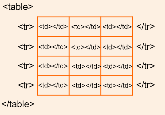
Simple feature collection with 4 features and 1 field
Geometry type: POINT
Dimension:     XY
Bounding box:  xmin: 1 ymin: 1 xmax: 2 ymax: 2
CRS:           NA
  feature    geometry
1       1 POINT (1 1)
2       2 POINT (1 2)
3       1 POINT (2 2)
4       2 POINT (2 1)

ระบบจุดอ้างอิง

• ข้อมูลเชิงพื้นที่ทั้งหมดต้องมีระบบการอ้างอิงพิกัด (CRS) เพื่อระบุตำแหน่งพิกัดบนโลก
• รายละเอียดเชิงฐานธรณีส่วนใหญ่ไม่จำเป็น แต่เสมอๆ มันดีที่ควรรู้ความแตกต่างระดับพื้นฐาน
  • ระบบการอ้างอิงพิกัดเชิงฐานธรณี (Geodetic CRS)
    • ใช้หน่วยมุม (องศา) เพราะมีพื้นฐานอยู่บนรูปทรงวงกลม
    • ส่วนใหญ่ใช้สำหรับการแสดงผลที่มีขนาดระดับโลกหรือระดับประเทศ
    • ตัวอย่าง: WGS84 (ระบบฐานธรณีโลก)
  • ระบบการอ้างอิงพิกัดที่ถูกฉาย (Projected CRS)
    • ใช้หน่วยเมตร (เมตร) เพราะมีพื้นฐานจากการฉายแบบของโลก
    • ส่วนใหญ่ใช้สำหรับการวิเคราะห์และการแสดงผลเชิงพื้นที่ที่มีความแม่นยำสูงในระดับภูมิภาคหรือระดับท้องที่
    • ตัวอย่าง: UTM (Universal Transversal Mercator)

UTM (Universal Transversal Mercator) - ระบบพิกัดที่ถูกฉาย แต่ละโซนเป็น CRS

EPSG codes

• CRS สามารถอ้างอิงได้โดยใช้รหัสตัวเลขที่เรียกว่ารหัส EPSG
  • EPSG database: https://epsg.io/, e.g. EPSG code 4326: https://epsg.io/4326

Some common CRS

Name	EPSG code	Area	Geodetic?	Use
World Geodetic System 1984 (WGS84)	4326	World	Yes	Basic geographic coordinates, common usage in GPS systems
WGS 84 / Pseudo-Mercator	3857	World	No	Google Maps, OpenStreetMap, general web mapping
UTM zone 32N	25832	Central Europe	No	Spatial analysis and measuring in Central Europe
LAEA Europe	3035	Europe	No	Multi-purpose CRS developed by the EU

CRS ใน R

• เราจะทำงานกับ CRS ใน R อย่างไร
  • แปลงเป็น dataframe แบบ sf: st_as_sf(..., crs = 4326)
  • กำหนด CRS ให้กับ dataframe แบบ sf ที่มีอยู่แล้ว: st_crs(...) <- 4326 หรือ st_set_crs(…, 4326)
  • เปลี่ยนแปลง CRS ที่มีอยู่แล้วเป็น CRS ใหม่: st_transform(..., 4326)

การจัดการกับชุดข้อมูล Guerry

• มาดูกันเรื่อง data_guerry และวิธีจัดการกับมันในรูปแบบ dataframe เชิงพื้นที่
• Guerry::gfrance85 มาในรูปแบบ sp dataframe ซึ่งถือว่าเก่า ดังนั้นเราต้องแปลงมัน
• ชุดข้อมูลนี้ยังมี CRS ที่ไม่ถูกต้องด้วย ดังนั้นเราต้องแก้ไขมัน

1data_guerry <- Guerry::gfrance85 %>%
2  st_as_sf() %>%
3  as_tibble() %>%
4  st_as_sf(crs = 27572) %>%
5  mutate(Region = case_match(
    Region,
    "C" ~ "Central",
    "E" ~ "East",
    "N" ~ "North",
    "S" ~ "South",
    "W" ~ "West"
  )) %>%
  select(-c("COUNT", "dept", "AVE_ID_GEO", "CODE_DEPT")) %>% # drop columns
  select(Region:Department, all_of(names(variable_names))) # select columns

1

Guerry::gfrance85 มาในรูปแบบวัตถุ sp และไม่มีข้อมูล CRS

2

… ดังนั้นเราแปลงมันเป็น dataframe แบบ sf

3

แปลงมันเป็น tibble เพื่อให้มันดูดีขึ้น(มั้ง)

4

สุดท้าย แปลงมันกลับไปเป็น sf และตั้งค่า CRS เป็น 25572 (ซึ่งเป็น CRS ของชุดข้อมูล Guerry เดิม)

5

ที่นี่ เราเปลี่ยนรหัสภูมิภาคที่สามารถใช้สำหรับการรวมข้อมูลเชิงพื้นที่

การดำเนินการทางพื้นที่

• เพื่อทำการmapข้อมูล Guerry เพิ่มความน่าสนใจคือการดำเนินการรวมข้อมูลทางพื้นที่เพื่อเปรียบเทียบข้อมูลในระดับภูมิภาคทางภูมิศาสตร์
• การดำเนินการทางพื้นที่ เช่น การรวมข้อมูลทางพื้นที่ เป็นหนึ่งในข้อได้เปรียบหลักของข้อมูลทางพื้นที่เมื่อเปรียบเทียบกับข้อมูลปกติ
• ใน Guerry เรามี2ระดับ: แผนก (ระดับเล็ก) และภูมิภาค (ระดับใหญ่)
• ในช่วงต่อไปเราจะดำเนินการรวมข้อมูลทางพื้นที่ นอก ฟังก์ชันserver

data_guerry_region <- data_guerry %>%
1    group_by(Region) %>%
2    summarise(across(
        .cols = all_of(names(variable_names)),
        function(x) {
            if (cur_column() %in% c("Area", "Pop1831")) {
                sum(x)
            } else {
                mean(x)
            }
        }
    ))

1

กำหนดกลุ่มตัวแปร (Region)

2

รวมตัวแปรและเรขาคณิตของ Guerry ตามตัวแปรกลุ่ม Region

ข้อมูลเชิงพื้นที่ Guerry

• คำถาม: เราสามารถบอกอะไรเกี่ยวกับชุดข้อมูล Guerry ในเรื่องของข้อมูลเชิงพื้นที่ได้บ้าง

data_guerry["Literacy"]

Simple feature collection with 85 features and 1 field
Geometry type: MULTIPOLYGON
Dimension:     XY
Bounding box:  xmin: 47680 ymin: 1703258 xmax: 1031401 ymax: 2677441
Projected CRS: NTF (Paris) / Lambert zone II
# A tibble: 85 × 2
   Literacy                                                             geometry
      <int>                                                   <MULTIPOLYGON [m]>
 1       37 (((801150 2092615, 800669 2093190, 800688 2095430, 800780 2095795, …
 2       51 (((729326 2521619, 729320 2521230, 729280 2518544, 728751 2517520, …
 3       13 (((710830 2137350, 711746 2136617, 712430 2135212, 712070 2134132, …
 4       46 (((882701 1920024, 882408 1920733, 881778 1921200, 881526 1922332, …
 5       69 (((886504 1922890, 885733 1922978, 885479 1923276, 883061 1925266, …
 6       27 (((747008 1925789, 746630 1925762, 745723 1925138, 744216 1925236, …
 7       67 (((818893 2514767, 818614 2514515, 817900 2514467, 817327 2514945, …
 8       18 (((509103 1747787, 508820 1747513, 508154 1747093, 505861 1746627, …
 9       59 (((775400 2345600, 775068 2345397, 773587 2345177, 772940 2344780, …
10       34 (((626230 1810121, 626269 1810496, 627494 1811321, 627681 1812424, …
# ℹ 75 more rows

แบบฝึกหัด

แบบฝึกหัด 1

ดึงวัตถุ sfc ออกมาจากชุดข้อมูล Guerry ความแตกต่างระหว่าง sf กับ sfc คืออะไร

Tip

ดูเอกสารคำสั่ง st_geometry()

Solution

st_geometry(data_guerry)

วัตถุ sf เป็น dataframes ที่ประกอบด้วย non-spatial featureคอลัมน์ และgeometry columnที่มีวัตถุ sfc

วัตถุ sfc คือการแสดงภาพของรูปทรงเชิงพื้นที่ พวกมันมีข้อมูล metadata เชิงพื้นที่ที่เกี่ยวข้องทั้งหมด

แบบฝึกหัด 2

ดึงวัตถุ sfg ลำดับที่ห้าออกมาจากวัตถุ sfc จากแบบฝึกหัด 1 ความแตกต่างระหว่างสองวัตถุเหล่านี้คืออะไร

Tip

วัตถุที่มีคลาสเป็น sfc ทำงานเหมือนกับ listและสามารถแบ่งย่อยได้ในลักษณะเดียวกัน

Solution

geom <- st_geometry(data_guerry)
geom[[1]]

วัตถุ sfg ประกอบด้วยรูปทรงเชิงพื้นที่ขั้นพื้นฐานซึ่งประกอบไปด้วยพิกัดเท่านั้น และทางเรขาคณิต (เช่น วิธีเชื่อมต่อพิกัดเพื่อสร้างรูปหลายเหลี่ยม)

วัตถุ sfc มีข้อมูล metadata เชิงพื้นที่ ซึ่งรวมถึง CRS ทำให้เราสามารถระบุตำแหน่งของพิกัดบนโลกได้

แบบฝึกหัด 3

data_guerry ประกอบด้วยรูปหลายเหลี่ยมหลายรูปทรง เราจะแปลงรูปเหลี่ยมเหล่านี้เป็นรูปจุดได้อย่างไร ลองดูที่ การอ้างอิงฟังก์ชัน ของแพ็คเกจ sf และค้นหาฟังก์ชัน (มีคำตอบหลายรูปแบบ) ที่สามารถแปลงรูปเหลี่ยมเป็นจุดๆได้

Tip

การค้นหาด้วยคำว่า “จุด” สามารถให้เห็นฟังก์ชันที่เหมาะที่สุดสำหรับการทำงานนี้ แต่ยังมีเยอะหลายวิธี

Solution

st_point_on_surface(data_guerry) ส่งคืนจุดที่มั่นใจว่าอยู่บนรูปหลายเหลี่ยม

st_centroid(data_guerry) ส่งคืนศูนย์กลางทางเรขาคณิตของรูปหลายเหลี่ยม

st_cast(data_guerry, "POINT") หรือ st_cast(data_guerry, "MULTIPOINT")

ทั้งหมดมันส่งคืนข้อความเตือน! ทำไมถึงเป็นเช่นนั้น?

st_sample(data_guerry, size = rep(1, nrow(data_guerry)))

ไม่ส่งคืนข้อความเตือน แต่เป็นแบบสุ่มและตัดทุกคุณสมบัติ

แบบฝึกหัด 4

ในขณะนี้ dataframe Guerry มี CRS เป็น “NTF (Paris) / Lambert zone II” ซึ่งเป็นการเลือกใช้ที่ดีแล้ว แต่มี CRS อื่น ๆ ที่อาจเป็นตัวเลือกที่ดีสำหรับการทำแผนที่ในฝรั่งเศสที่แม่นยำอีกหรือไม่

Tip

จำระบบพิกัด UTM ไว้ เลื่อนขึ้นไปดู UTM zones ที่แล้ว

Solution

แม้ว่าจะมี CRS หลายตัวที่อาจเป็นตัวเลือกที่ดี แต่หนึ่งในการแก้ไขที่เราได้พูดถึงในworkshopนี้คือ UTM zones เมื่อดูที่ภาพของเขต UTM เราสามารถเห็นได้ว่า UTM 31N zones มันครอบคลุมพื้นที่ของฝรั่งเศสเกือบทั้งหมด

แบบฝึกหัด 5

แปลง dataframe Guerry ให้เป็น CRS ใหม่จากแบบฝึกหัดที่ 4

Tip

จำไว้ว่าเราเปิด https://epsg.io/ เพื่อค้นหารหัส EPSG ได้

Solution

โดยใช้ฟังก์ชันค้นหาจาก epsg.io เราสามารถระบุได้ว่ารหัส EPSG ที่ใช้แปลงชุดข้อมูล Guerry จาก Lambert zone II ไปยัง UTM zone 31N คือ 23031, 25831 หรือ 32631

  st_transform(data_guerry, 23031)

การสร้างแผนที่แบบโต้ตอบด้วย Leaflet

• R ให้บริการหลายวิธีในการสร้างแผนที่ บางวิธีก็มีความซับซ้อนมากกว่าบางวิธี

  • ggplot2 สนับสนุนข้อมูลเชิงพื้นที่ด้วยฟังก์ชันเช่น geom_sf, coord_sf และฟังก์ชันที่กำหนดเองเช่น stars::geom_stars
  • tmap เป็นกรอบงานที่ครอบคลุมสำหรับการสร้างแผนที่ธีมที่มีคุณภาพสูง
  • cartography และ mapsf รวมหลักการการทำแผนที่เข้าด้วยกัน ทำให้ R ทำงานได้ใกล้เคียงกับซอฟต์แวร์สร้างแผนที่โดยเฉพาะ
  • leaflet ทำการเชื่อมต่อกับไลบรารี JavaScript ของ Leaflet เพื่อสร้างการแสดงผลแผนที่แบบโต้ตอบ

การผสมผสาน Leaflet ใน Shiny

• Leaflet ใน Shiny ทำงานเหมือนกับการแสดงผลประเภทอื่น ๆ เราต้องการ:
  • ผลลัพธ์ของ UI: leaflet::leafletOutput()
  • ฟังก์ชันการเรนเดอร์: leaflet::renderLeaflet()
• ในแอพของเรา เราเพิ่มตัวสำรวจเชิงภูมิศาสตร์ของชุดข้อมูล Guerry

1tabItem(
  tabName = "tab_map",
2  fluidRow(
    column(
      width = 12,
      box(
        id = "tab_map_box",
        status = "primary",
        headerBorder = FALSE,
        collapsible = FALSE,
        width = 12,
3        leaflet::leafletOutput("tab_map_map", height = "800px", width = "100%")
      ) # end box
    ) # end column
  ) # end fluidRow
) # end tabItem

1

สร้างแท็บใหม่ชื่อว่า tab_map

2

เพิ่ม fluid row ที่มีคอลัมน์และกล่องที่ครอบคลุมทั้งหน้า

3

เพิ่มoutput ของ UI ที่จะรองรับแผนที่ของ leaflet ที่ครอบคลุมความกว้างทั้งหมดและมีความสูง 800 พิกเซล

หัวใจของ Leaflet

• แพ็กเกจ leaflet ขึ้นกับฟังก์ชันหลัก leaflet() ซึ่งสร้างแผนที่เปล่า
• ฟังก์ชันเพิ่มเติมทุกฟังก์ชันสามารถเพิ่มเข้าไปเสริมส่วนการแสดงผลแผนที่เพิ่มเติมได้ (คล้ายกับ ggplot2)
  • addProviderTiles() เพิ่มแผนที่พื้นฐาน, ในกรณีนี้เราใช้แผนที่พื้นฐานสี่แผนที่ที่สามารถเลือกได้
  • addLayersControl() เพิ่มปุ่มที่ช่วยให้เราสามารถสลับระหว่างlayerข้อมูลแผนที่
  • setView() ตั้งค่าศูนย์กลางและระดับซูมของมุมมองแผนที่

1output$tab_map_map <- leaflet::renderLeaflet({
2        leaflet() %>%
3            addProviderTiles("OpenStreetMap.France", group = "OSM") %>%
            addProviderTiles("OpenTopoMap", group = "OTM") %>%
            addProviderTiles("Stamen.TonerLite", group = "Stamen Toner") %>%
            addProviderTiles("GeoportailFrance.orthos", group = "Orthophotos") %>%
4            addLayersControl(baseGroups = c("OSM", "OTM",
                                                                            "Stamen Toner", "Orthophotos")) %>%
5            setView(lng = 3, lat = 47, zoom = 5)
})

1

เติมผลลัพธ์ tab_map_map ด้วยแผนที่ leaflet โดยใช้ renderLeaflet

2

เพิ่มแผนที่เปล่าโดยใช้ leaflet()

3

เพิ่มแผนที่พื้นฐานหลายแผนที่: OpenStreetMap, OpenTopoMap, Stamen และortho photos จาก geo portal ฝรั่งเศส

4

เพิ่มปุ่มเพื่อควบคุมว่าต้องการแสดงแผนที่พื้นฐานอันไหน

5

ตั้งค่าศูนย์กลางของแผนที่และระดับซูมเริ่มต้น

Full code

Full code including an empty map

library(shiny)
library(htmltools)
library(bs4Dash)
library(fresh)
library(waiter)
library(shinyWidgets)
library(Guerry)
library(sf)
library(tidyr)
library(dplyr)
library(RColorBrewer)
library(viridis)
library(leaflet)
library(plotly)
library(ggplot2)
library(GGally)
library(datawizard)
library(parameters)
library(performance)
library(modelsummary)

# 1 Data preparation ----

## Load & clean data ----
variable_names <- list(
  Crime_pers = "Crime against persons",  
  Crime_prop =  "Crime against property",  
  Literacy = "Literacy",  
  Donations = "Donations to the poor",  
  Infants = "Illegitimate births",  
  Suicides = "Suicides",  
  Wealth = "Tax / capita",  
  Commerce = "Commerce & Industry",  
  Clergy = "Clergy",  
  Crime_parents = "Crime against parents",  
  Infanticide = "Infanticides",  
  Donation_clergy = "Donations to the clergy",  
  Lottery = "Wager on Royal Lottery",  
  Desertion = "Military desertion",  
  Instruction = "Instruction",  
  Prostitutes = "Prostitutes",  
  Distance = "Distance to paris",  
  Area = "Area",  
  Pop1831 = "Population"
)

variable_desc <- list(
  Crime_pers = list(
    title = "Crime against persons",
    desc = as.character(p(tags$b("Crime against persons:"), "Population per crime against persons", hr(), helpText("Source: Table A2 in Guerry (1833). Compte général, 1825-1830"))),
    lgd = "Pop. per crime",
    unit = ""
  ),
  Crime_prop = list(
    title = "Crime against property",
    desc = as.character(p(tags$b("Crime against property:"), "Population per crime against property", hr(), helpText("Source: Compte général, 1825-1830"))),
    lgd = "Pop. per crime",
    unit = ""
  ),
  Literacy = list(
    title = "Literacy",
    desc = as.character(p(tags$b("Percent Read & Write:"), "Percent of military conscripts who can read and write", hr(), helpText("Source: Table A2 in Guerry (1833)"))),
    lgd = "Literacy",
    unit = " %"
  ),
  Donations = list(
    title = "Donations to the poor",
    desc = as.character(p(tags$b("Donations to the poor"), hr(), helpText("Source: Table A2 in Guerry (1833). Bulletin des lois"))),
    lgd = "Donations",
    unit = ""
  ),
  Infants = list(
    title = "Illegitimate births",
    desc = as.character(p(tags$b("Population per illegitimate birth"), hr(), helpText("Source: Table A2 in Guerry (1833). Bureau des Longitudes, 1817-1821"))),
    lgd = "Pop. per birth",
    unit = ""
  ),
  Suicides = list(
    title = "Suicides",
    desc = as.character(p(tags$b("Population per suicide"), hr(), helpText("Source: Table A2 in Guerry (1833). Compte général, 1827-1830"))),
    lgd = "Pop. per suicide",
    unit = ""
  ),
  Wealth = list(
    title = "Tax / capita",
    desc = as.character(p(tags$b("Per capita tax on personal property:"), "A ranked index based on taxes on personal and movable property per inhabitant", hr(), helpText("Source: Table A1 in Guerry (1833)"))),
    lgd = "Tax / capita",
    unit = ""
  ),
  Commerce = list(
    title = "Commerce & Industry",
    desc = as.character(p(tags$b("Commerce & Industry:"), "Commerce and Industry, measured by the rank of the number of patents / population", hr(), helpText("Source: Table A1 in Guerry (1833)"))),
    lgd = "Patents / capita",
    unit = ""
  ),
  Clergy = list(
    title = "Clergy",
    desc = as.character(p(tags$b("Distribution of clergy:"), "Distribution of clergy, measured by the rank of the number of Catholic priests in active service / population", hr(), helpText("Source: Table A1 in Guerry (1833). Almanach officiel du clergy, 1829"))),
    lgd = "Priests / capita",
    unit = ""
  ),
  Crime_parents = list(
    title = "Crime against parents",
    desc = as.character(p(tags$b("Crime against parents:"), "Crimes against parents, measured by the rank of the ratio of crimes against parents to all crimes \u2013 Average for the years 1825-1830", hr(), helpText("Source: Table A1 in Guerry (1833). Compte général"))),
    lgd = "Share of crimes",
    unit = " %"
  ),
  Infanticide = list(
    title = "Infanticides",
    desc = as.character(p(tags$b("Infanticides per capita:"), "Ranked ratio of number of infanticides to population \u2013 Average for the years 1825-1830", hr(), helpText("Source: Table A1 in Guerry (1833). Compte général"))),
    lgd = "Infanticides / capita",
    unit = ""
  ),
  Donation_clergy = list(
    title = "Donations to the clergy",
    desc = as.character(p(tags$b("Donations to the clergy:"), "Ranked ratios of the number of bequests and donations inter vivios to population \u2013 Average for the years 1815-1824", hr(), helpText("Source: Table A1 in Guerry (1833). Bull. des lois, ordunn. d’autorisation"))),
    lgd = "Donations / capita",
    unit = ""
  ),
  Lottery = list(
    title = "Wager on Royal Lottery",
    desc = as.character(p(tags$b("Per capita wager on Royal Lottery:"), "Ranked ratio of the proceeds bet on the royal lottery to population \u2013 Average for the years 1822-1826", hr(), helpText("Source: Table A1 in Guerry (1833). Compte rendu par le ministre des finances"))),
    lgd = "Wager / capita",
    unit = ""
  ),
  Desertion = list(
    title = "Military desertion",
    desc = as.character(p(tags$b("Military desertion:"), "Military disertion, ratio of the number of young soldiers accused of desertion to the force of the military contingent, minus the deficit produced by the insufficiency of available billets\u2013 Average of the years 1825-1827", hr(), helpText("Source: Table A1 in Guerry (1833). Compte du ministère du guerre, 1829 état V"))),
    lgd = "No. of desertions",
    unit = ""
  ),
  Instruction = list(
    title = "Instruction",
    desc = as.character(p(tags$b("Instruction:"), "Ranks recorded from Guerry's map of Instruction. Note: this is inversely related to literacy (as defined here)")),
    lgd = "Instruction",
    unit = ""
  ),
  Prostitutes = list(
    title = "Prostitutes",
    desc = as.character(p(tags$b("Prostitutes in Paris:"), "Number of prostitutes registered in Paris from 1816 to 1834, classified by the department of their birth", hr(), helpText("Source: Parent-Duchatelet (1836), De la prostitution en Paris"))),
    lgd = "No. of prostitutes",
    unit = ""
  ),
  Distance = list(
    title = "Distance to paris",
    desc = as.character(p(tags$b("Distance to Paris (km):"), "Distance of each department centroid to the centroid of the Seine (Paris)", hr(), helpText("Source: Calculated from department centroids"))),
    lgd = "Distance",
    unit = " km"
  ),
  Area = list(
    title = "Area",
    desc = as.character(p(tags$b("Area (1000 km\u00b2)"), hr(), helpText("Source: Angeville (1836)"))),
    lgd = "Area",
    unit = " km\u00b2"
  ),
  Pop1831 = list(
    title = "Population",
    desc = as.character(p(tags$b("Population in 1831, in 1000s"), hr(), helpText("Source: Taken from Angeville (1836), Essai sur la Statistique de la Population français"))),
    lgd = "Population (in 1000s)",
    unit = ""
  )
)

data_guerry <- Guerry::gfrance85 %>%
  st_as_sf() %>%
  as_tibble() %>%
  st_as_sf(crs = 27572) %>%
  mutate(Region = case_match(
    Region,
    "C" ~ "Central",
    "E" ~ "East",
    "N" ~ "North",
    "S" ~ "South",
    "W" ~ "West"
  )) %>%
  select(-c("COUNT", "dept", "AVE_ID_GEO", "CODE_DEPT")) %>%
  select(Region:Department, all_of(names(variable_names)))



## Prep data (Tab: Tabulate data) ----
data_guerry_tabulate <- data_guerry %>% 
  st_drop_geometry() %>% 
  mutate(across(.cols = all_of(names(variable_names)), round, 2))


## Prep data (Tab: Map data) ----
data_guerry_region <- data_guerry %>%
  group_by(Region) %>%
  summarise(across(
    .cols = all_of(names(variable_names)),
    function(x) {
      if (cur_column() %in% c("Area", "Pop1831")) {
        sum(x)
      } else {
        mean(x)
      }
    }
  ))

## Prepare palettes ----
## Used for mapping
pals <- list(
  Sequential = RColorBrewer::brewer.pal.info %>%
    filter(category %in% "seq") %>%
    row.names(),
  Viridis = c("Magma", "Inferno", "Plasma", "Viridis",
              "Cividis", "Rocket", "Mako", "Turbo")
)

## Prepare modebar clean-up ----
## Used for modelling
plotly_buttons <- c(
  "sendDataToCloud", "zoom2d", "select2d", "lasso2d", "autoScale2d",
  "hoverClosestCartesian", "hoverCompareCartesian", "resetScale2d"
)




# 3 UI ----

ui <- dashboardPage(
  title = "The Guerry Dashboard",
  ## 3.1 Header ----
  header = dashboardHeader(
    title = tagList(
      img(src = "../workshop-logo.png", width = 35, height = 35),
      span("The Guerry Dashboard", class = "brand-text")
    )
  ),
  ## 3.2 Sidebar ----
  sidebar = dashboardSidebar(
    id = "sidebar",
    sidebarMenu(
      id = "sidebarMenu",
      menuItem(tabName = "tab_intro", text = "Introduction", icon = icon("home")),
      menuItem(tabName = "tab_tabulate", text = "Tabulate data", icon = icon("table")),
      menuItem(tabName = "tab_model", text = "Model data", icon = icon("chart-line")),
      menuItem(tabName = "tab_map", text = "Map data", icon = icon("map")),
      flat = TRUE
    ),
    minified = TRUE,
    collapsed = TRUE,
    fixed = FALSE,
    skin = "light"
  ),
  ## 3.3 Body ----
  body = dashboardBody(
    tabItems(
      ### 3.1.1 Tab: Introduction ----
      tabItem(
        tabName = "tab_intro",
        jumbotron(
          title = "The Guerry Dashboard",
          lead = "A Shiny app to explore the classic Guerry dataset.",
          status = "info",
          btnName = NULL
        ),
        fluidRow(
          column(width = 1),
          column(
            width = 6,
            box(
              title = "About",
              status = "primary",
              width = 12,
              blockQuote(HTML("André-Michel Guerry was a French lawyer and
                          amateur statistician. Together with Adolphe
                          Quetelet he may be regarded as the founder of
                          moral statistics which led to the development
                          of criminology, sociology and ultimately,
                          modern social science. <br>— Wikipedia: <a href='https://en.wikipedia.org/wiki/Andr%C3%A9-Michel_Guerry'>André-Michel Guerry</a>"),
                         color = "primary"),
              p(HTML("Andre-Michel Guerry (1833) was the first to 
              systematically collect and analyze social data 
               on such things as crime, literacy and suicide 
               with the view to determining social laws and the 
               relations among these variables. The Guerry data 
               frame comprises a collection of 'moral variables' 
               (cf. <i><a href='https://en.wikipedia.org/wiki/Moral_statistics'>moral statistics</a></i>) 
               on the 86 departments of France around 1830. 
               A few additional variables have been added 
               from other sources. In total the data frame has 
               86 observations (the departments of France) on 23 variables <i>(Source: <code>?Guerry</code>)</i>. 
               In this app, we aim to explore Guerry’s data
                using spatial exploration and regression modelling.")),
              hr(),
              accordion(
                id = "accord",
                accordionItem(
                  title = "References",
                  status = "primary",
                  solidHeader = FALSE,
                  "The following sources are referenced in this app:",
                  tags$ul(
                    class = "list-style: none",
                    style = "margin-left: -30px;",
                    p("Angeville, A. (1836). Essai sur la Statistique de la Population française Paris: F. Doufour."),
                    p("Guerry, A.-M. (1833). Essai sur la statistique morale de la France Paris: Crochard. English translation: Hugh P. Whitt and Victor W. Reinking, Lewiston, N.Y. : Edwin Mellen Press, 2002."),
                    p("Parent-Duchatelet, A. (1836). De la prostitution dans la ville de Paris, 3rd ed, 1857, p. 32, 36"),
                    p("Palsky, G. (2008). Connections and exchanges in European thematic cartography. The case of 19th century choropleth maps. Belgeo 3-4, 413-426.")
                  )
                ),
                accordionItem(
                  title = "Details",
                  status = "primary",
                  solidHeader = FALSE,
                  p("This app was created as part of a Shiny workshop held in July 2023"),
                  p("Last update: June 2023"),
                  p("Further information about the data can be found",
                    a("here.", href = "https://www.datavis.ca/gallery/guerry/guerrydat.html"))
                )
              )
            )
          ),
          column(
            width = 4,
            box(
              title = "André Michel Guerry",
              status = "primary",
              width = 12,
              tags$img(src = "../guerry.jpg", width = "100%"),
              p("Source: Palsky (2008)")
            )
          )
        )
      ),
      ### 3.3.2 Tab: Tabulate data ----
      tabItem(
        tabName = "tab_tabulate",
        fluidRow(
          #### Inputs(s) ----
          pickerInput(
            "tab_tabulate_select",
            label = "Filter variables",
            choices = setNames(names(variable_names), variable_names),
            options = pickerOptions(
              actionsBox = TRUE,
              windowPadding = c(30, 0, 0, 0),
              liveSearch = TRUE,
              selectedTextFormat = "count",
              countSelectedText = "{0} variables selected",
              noneSelectedText = "No filters applied"
            ),
            inline = TRUE,
            multiple = TRUE
          )
        ),
        hr(),
        #### Output(s) (Data table) ----
        DT::dataTableOutput("tab_tabulate_table")
      ),
      ### 3.3.3 Tab: Model data ----
      tabItem(
        tabName = "tab_model",
        fluidRow(
          column(
            width = 6,
            #### Inputs(s) ----
            box(
              width = 12,
              title = "Select variables",
              status = "primary",
              shinyWidgets::pickerInput(
                "model_x",
                label = "Select a dependent variable",
                choices = setNames(names(variable_names), variable_names),
                options = shinyWidgets::pickerOptions(liveSearch = TRUE),
                selected = "Literacy"
              ),
              shinyWidgets::pickerInput(
                "model_y",
                label = "Select independent variables",
                choices = setNames(names(variable_names), variable_names),
                options = shinyWidgets::pickerOptions(
                  actionsBox = TRUE,
                  liveSearch = TRUE,
                  selectedTextFormat = "count",
                  countSelectedText = "{0} variables selected",
                  noneSelectedText = "No variables selected"
                ),
                multiple = TRUE,
                selected = "Commerce"
              ),
              shinyWidgets::prettyCheckbox(
                "model_std",
                label = "Standardize variables?",
                value = TRUE,
                status = "primary",
                shape = "curve"
              ),
              hr(),
              actionButton(
                "refresh",
                label = "Apply changes",
                icon = icon("refresh"),
                flat = TRUE
              )
            ),
            #### Outputs(s) ----
            tabBox(
              status = "primary",
              type = "tabs",
              title = "Model analysis",
              side = "right",
              width = 12,
              ##### Tabpanel: Coefficient plot ----
              tabPanel(
                title = "Plot: Coefficients",
                plotly::plotlyOutput("coefficientplot")
              ),
              ##### Tabpanel: Scatterplot ----
              tabPanel(
                title = "Plot: Scatterplot",
                plotly::plotlyOutput("scatterplot")
              ),
              ##### Tabpanel: Table: Regression ----
              tabPanel(
                title = "Table: Model",
                htmlOutput("tableregression")
              )
            )
          ),
          column(
            width = 6,
            ##### Box: Pair diagramm ----
            box(
              width = 12,
              title = "Pair diagram",
              status = "primary",
              plotly::plotlyOutput("pairplot")
            ),
            ##### TabBox: Model diagnostics ----
            tabBox(
              status = "primary",
              type = "tabs",
              title = "Model diagnostics",
              width = 12,
              side = "right",
              tabPanel(
                title = "Normality",
                plotly::plotlyOutput("normality")
              ),
              tabPanel(
                title = "Outliers",
                plotly::plotlyOutput("outliers")
              ),
              tabPanel(
                title = "Heteroskedasticity",
                plotly::plotlyOutput("heteroskedasticity")
              )
            )
          )
        )
      ),
      ### 3.3.4 Tab: Map data ----
      tabItem(
        tabName = "tab_map", # must correspond to related menuItem name
        fluidRow(
          column(
            #### Output(s) ----
            width = 8,
            box(
              id = "tab_map_box",
              status = "primary",
              headerBorder = FALSE,
              collapsible = FALSE,
              width = 12,
              leaflet::leafletOutput("tab_map_map", height = "800px", width = "100%")
            ) # end box
          ) # end column
        ) # end fluidRow
      ) # end tabItem
    ) # end tabItems
  ),
  
  ## 3.4 Footer (bottom)----
  footer = dashboardFooter(
    left = span(
      "This dashboard was created by Jonas Lieth and Paul Bauer. Find the source code",
      a("here.", href = "https://github.com/paulcbauer/shiny_workshop/tree/main/shinyapps/guerry"),
      "It is based on data from the",
      a("Guerry R package.", href = "https://cran.r-project.org/web/packages/Guerry/index.html")
    )
  ),
  ## 3.5 Controlbar (top)----
  controlbar = dashboardControlbar(
    div(class = "p-3", skinSelector()),
    skin = "light"
  )  
)



# 4 Server ----

server <- function(input, output, session) {
  
  ## 4.1 Tabulate data ----
  ### Variable selection ----
  tab <- reactive({
    var <- input$tab_tabulate_select
    data_table <- data_guerry_tabulate
    
    if (!is.null(var)) {
      data_table <- data_table[, var]
    }
    
    data_table
  })
  
  
  ### Create table----
  dt <- reactive({
    tab <- tab()
    ridx <- ifelse("Department" %in% names(tab), 3, 1)
    DT::datatable(
      tab,
      class = "hover",
      extensions = c("Buttons"),
      selection = "none",
      filter = list(position = "top", clear = FALSE),
      style = "bootstrap4",
      rownames = FALSE,
      options = list(
        dom = "Brtip",
        deferRender = TRUE,
        scroller = TRUE,
        buttons = list(
          list(extend = "copy", text = "Copy to clipboard"),
          list(extend = "pdf", text = "Save as PDF"),
          list(extend = "csv", text = "Save as CSV"),
          list(extend = "excel", text = "Save as JSON", action = DT::JS("
          function (e, dt, button, config) {
            var data = dt.buttons.exportData();
  
            $.fn.dataTable.fileSave(
              new Blob([JSON.stringify(data)]),
              'Shiny dashboard.json'
            );
          }
        "))
        )
      )
    )
  })
  
  ### Render table----
  output$tab_tabulate_table <- DT::renderDataTable(dt(), server = FALSE)
  
  
  
  ## 4.2 Model data ----
  ### Define & estimate model ----
  mparams <- reactive({
    x <- input$model_x
    y <- input$model_y
    dt <- sf::st_drop_geometry(data_guerry)[c(x, y)]
    dt_labels <- sf::st_drop_geometry(data_guerry)[c("Department", "Region")]
    if (input$model_std) dt <- datawizard::standardise(dt)
    form <- as.formula(paste(x, "~", paste(y, collapse = " + ")))
    mod <- lm(form, data = dt)
    
    list(
      x = x,
      y = y,
      data = dt,
      data_labels = dt_labels,
      model = mod
    )
  }) %>%
    bindEvent(input$refresh, ignoreNULL = FALSE)
  
  ### Pair diagram ----
  output$pairplot <- plotly::renderPlotly({
    params <- mparams()
    dt <- params$data
    dt_labels <- params$data_labels
    p <- GGally::ggpairs(
      params$data,
      axisLabels = "none",
      lower = list(
        continuous = function(data, mapping, ...) {
          ggplot(data, mapping) +
            suppressWarnings(geom_point(
              aes(text = paste0(
                "Department: ", 
                dt_labels[["Department"]],
                "<br>Region: ", 
                dt_labels[["Region"]])),
              color = "black"
            ))
        }
      )
    )
    if (isTRUE(input$dark_mode)) p <- p +
      dark_theme_gray() +
      theme(plot.background = element_rect(fill = "#343a40"))
    ggplotly(p) %>%
      config(modeBarButtonsToRemove = plotly_buttons,
             displaylogo = FALSE)
  })
  
  ### Plot: Coefficientplot ----
  output$coefficientplot <- renderPlotly({
    params <- mparams()
    dt <- params$data
    x <- params$x
    y <- params$y
    
    
    p <- plot(parameters::model_parameters(params$model))
    
    if (isTRUE(input$dark_mode)) p <- p +
      geom_point(color = "white") +
      dark_theme_gray() +
      theme(plot.background = element_rect(fill = "#343a40"))
    ggplotly(p) %>%
      config(modeBarButtonsToRemove = plotly_buttons,
             displaylogo = FALSE)
  })
  
  ### Plot: Scatterplot ----
  output$scatterplot <- renderPlotly({
    params <- mparams()
    dt <- params$data
    dt_labels <- params$data_labels
    x <- params$x 
    y <- params$y
    
    
    if (length(y) == 1) {
      p <- ggplot(params$data, 
                  aes(x = .data[[params$x]], 
                      y = .data[[params$y]])) +
        geom_point(aes(text = paste0("Department: ", 
                                     dt_labels[["Department"]],
                                     "<br>Region: ", 
                                     dt_labels[["Region"]])),
                   color = "black") +
        geom_smooth() + 
        geom_smooth(method='lm') +
        theme_light()
    } else {
      p <- ggplot() +
        theme_void() +
        annotate("text", 
                 label = "Cannot create scatterplot.\nMore than two variables selected.", 
                 x = 0, y = 0, 
                 size = 5, 
                 colour = "red",
                 hjust = 0.5,
                 vjust = 0.5) +
        xlab(NULL)
      
    }
    
    if (isTRUE(input$dark_mode)) p <- p +
      geom_point(color = "white") +
      dark_theme_gray() +
      theme(plot.background = element_rect(fill = "#343a40"))
    ggplotly(p) %>%
      config(modeBarButtonsToRemove = plotly_buttons,
             displaylogo = FALSE)
  })
  
  ### Table: Regression ----
  output$tableregression <- renderUI({
    params <- mparams()
    HTML(modelsummary(
      dvnames(list(params$model)),
      gof_omit = "AIC|BIC|Log|Adj|RMSE"
    ))
  })
  
  ### Plot: Normality residuals ----
  output$normality <- renderPlotly({
    params <- mparams()
    p <- plot(performance::check_normality(params$model))
    if (isTRUE(input$dark_mode)) p <- p +
      dark_theme_gray() +
      theme(plot.background = element_rect(fill = "#343a40"))
    ggplotly(p) %>%
      config(modeBarButtonsToRemove = plotly_buttons,
             displaylogo = FALSE)
  })
  
  ### Plot: Outliers ----
  output$outliers <- renderPlotly({
    params <- mparams()
    p <- plot(performance::check_outliers(params$model), show_labels = FALSE)
    if (isTRUE(input$dark_mode)) p <- p +
      dark_theme_gray() +
      theme(plot.background = element_rect(fill = "#343a40"))
    p$labels$x <- "Leverage"
    ggplotly(p) %>%
      config(modeBarButtonsToRemove = plotly_buttons,
             displaylogo = FALSE)
  })
  
  ### Plot: Heteroskedasticity ----
  output$heteroskedasticity <- renderPlotly({
    params <- mparams()
    p <- plot(performance::check_heteroskedasticity(params$model))
    if (isTRUE(input$dark_mode)) p <- p +
      dark_theme_gray() +
      theme(plot.background = element_rect(fill = "#343a40"))
    p$labels$y <- "Sqrt. |Std. residuals|" # ggplotly doesn't support expressions
    ggplotly(p) %>%
      config(modeBarButtonsToRemove = plotly_buttons,
             displaylogo = FALSE)
  })
  
  
  ## 4.3 Map data ----
  output$tab_map_map <- leaflet::renderLeaflet({
    leaflet() %>%
      addProviderTiles("OpenStreetMap.France", group = "OSM") %>%
      addProviderTiles("OpenTopoMap", group = "OTM") %>%
      addProviderTiles("Stamen.TonerLite", group = "Stamen Toner") %>%
      addProviderTiles("GeoportailFrance.orthos", group = "Orthophotos") %>%
      addLayersControl(baseGroups = c("OSM", "OTM",
                                      "Stamen Toner", "Orthophotos")) %>%
      setView(lng = 3, lat = 47, zoom = 5)
  })
}

shinyApp(ui, server)

เพิ่มข้อมูล

• ตอนนี้เราแสดงเฉพาะพื้นหลังเท่านั้น แต่ไม่ได้แสดงข้อมูล Guerry
• เพิ่มข้อมูลโดยใช้ฟังก์ชันชั้นข้อมูล เช่น:
  • addMarkers() เพิ่มข้อมูลจุด
  • addPolylines() เพิ่มข้อมูลเส้น
  • addPolygons() เพิ่มข้อมูลรูปหลายเหลี่ยม
  • addRasterImage() เพิ่มข้อมูลราสเตอร์
  • addLegend() เพิ่มคำอธิบาย

ปรับแต่งเฉพาะสำหรับแผนที่ Leaflet

• ตัวแปรถูกส่งผ่านโดยใช้สูตร (นั่นคือ แทนที่จะเขียน data_guerry$Literacy เราจะเขียน ~Literacy)
• โดยค่าเริ่มต้น Leaflet รองรับเฉพาะ WGS84 (EPSG:4326) เป็น CRS
• สีของข้อมูลจะถูกตั้งค่าโดยใช้ฟังก์ชันที่กำหนดเองซึ่งถูกสร้างในฟังก์ชัน:
  • colorNumeric() สำหรับแผนที่ค่าต่อเนื่อง
  • colorBin() สำหรับแผนที่ค่าต่อเนื่องที่ถูกแบ่งออกเป็นช่วงที่เท่ากัน
  • colorQuantile() สำหรับแผนที่ค่าต่อเนื่องที่ถูกแบ่งออกเป็นช่วงตามควอไทล์
  • colorFactor() สำหรับแผนที่ค่าหมวดหมู่
• highlightOptions() เพิ่มเอฟเฟคเด่นสว่างเมื่อวางเม้าส์เหนือรูปหลายเหลี่ยม

output$tab_map_map <- leaflet::renderLeaflet({
1    pal <- colorNumeric(palette = "Reds", domain = NULL)
    
2    leaflet(data = st_transform(data_guerry, 4326)) %>%
3        addProviderTiles("OpenStreetMap.France") %>%
4        setView(lng = 3, lat = 47, zoom = 5) %>%
5        addPolygons(
6            fillColor = ~params$pal(Literacy),
7            fillOpacity = 0.7,
            weight = 1,
            color = "black",
            opacity = 0.5,
8            highlightOptions = highlightOptions(
                weight = 2,
                color = "black",
                opacity = 0.5,
                fillOpacity = 1,
                bringToFront = TRUE,
                sendToBack = TRUE
            )
        ) %>%
9        addLegend(
            position = "bottomright",
10            pal = pal,
            values = ~Literacy,
            opacity = 0.9,
            title = "Literacy",
11            labFormat = labelFormat(suffix = " %")
        )
})

1

กำหนดสีสำหรับการสร้างแผนที่ ที่นี่เราต้องการแสดงค่าที่ต่อเนื่องในสีแดง ผลลัพธ์คือฟังก์ชันที่เรียกว่า pal() ซึ่งเราจะใช้ในภายหลัง

2

สร้างแผนที่เปล่า เพิ่มข้อมูลทางภูมิศาสตร์ โปรดทราบว่า Leaflet โดยค่าเริ่มต้นรับเฉพาะข้อมูลทางภูมิศาสตร์ที่มี EPSG:4326 สำหรับข้อมูลอื่นๆ โปรดอ้างอิงถึง leaflet::leafletCRS() แต่ไม่ควรคาดหวังว่าจะเข้าใจทุกอย่างที่เกิดขึ้น 555

3

เพิ่มแผนที่พื้นฐานของ OpenStreetMap ฝรั่งเศส

4

กำหนดศูนย์กลางและระดับการซูมของมุมมองเริ่มต้น

5

ฟังก์ชัน addPolygons() เพิ่มรูปหลายเหลี่ยมลงในแผนที่ Leaflet

6

fillColor กำหนดวิธีการระบายสีของรูปหลายเหลี่ยม เราส่งสูตรที่มีการเรียกใช้ฟังก์ชัน pal() ที่เราสร้างขึ้น (ดูข้อ 2) เพื่อแมปสีกับตัวแปร Literacy

7

เราสามารถเพิ่มพารามิเตอร์เพิ่มเติมที่ควบคุมการแสดงผลของแผนที่ เช่น ความทึบแสง, สี หรือความหนาของเส้น (น้ำหนัก)

8

highlightOptions() ช่วยให้สามารถเพิ่มเอฟเฟ็คเด่นสว่างเมื่อวางเม้าส์เหนือรูปหลายเหลี่ยม

9

โดยใช้ addLegend() เราเพิ่มคำอธิบายลงในแผนที่ Leaflet ที่มุมขวาล่าง

10

addLegend() รับค่าในลักษณะเดียวกับ addPolygons(): pal รับฟังก์ชันเก็บสีที่สร้างขึ้นและ values รับสูตรที่มีชื่อคอลัมน์ในinput dataset

11

สุดท้าย labelFormat() ช่วยให้เราสามารถเปลี่ยนรูปแบบของป้ายคำอธิบาย หากต้องการระบุว่าตัวเลขเป็นเปอร์เซ็นต์ เมตร หรืออื่น

Full code

Full code including a simple Leaflet map

library(shiny)
library(htmltools)
library(bs4Dash)
library(fresh)
library(waiter)
library(shinyWidgets)
library(Guerry)
library(sf)
library(tidyr)
library(dplyr)
library(RColorBrewer)
library(viridis)
library(leaflet)
library(plotly)
library(ggplot2)
library(GGally)
library(datawizard)
library(parameters)
library(performance)
library(modelsummary)

# 1 Data preparation ----

## Load & clean data ----
variable_names <- list(
  Crime_pers = "Crime against persons",  
  Crime_prop =  "Crime against property",  
  Literacy = "Literacy",  
  Donations = "Donations to the poor",  
  Infants = "Illegitimate births",  
  Suicides = "Suicides",  
  Wealth = "Tax / capita",  
  Commerce = "Commerce & Industry",  
  Clergy = "Clergy",  
  Crime_parents = "Crime against parents",  
  Infanticide = "Infanticides",  
  Donation_clergy = "Donations to the clergy",  
  Lottery = "Wager on Royal Lottery",  
  Desertion = "Military desertion",  
  Instruction = "Instruction",  
  Prostitutes = "Prostitutes",  
  Distance = "Distance to paris",  
  Area = "Area",  
  Pop1831 = "Population"
)

variable_desc <- list(
  Crime_pers = list(
    title = "Crime against persons",
    desc = as.character(p(tags$b("Crime against persons:"), "Population per crime against persons", hr(), helpText("Source: Table A2 in Guerry (1833). Compte général, 1825-1830"))),
    lgd = "Pop. per crime",
    unit = ""
  ),
  Crime_prop = list(
    title = "Crime against property",
    desc = as.character(p(tags$b("Crime against property:"), "Population per crime against property", hr(), helpText("Source: Compte général, 1825-1830"))),
    lgd = "Pop. per crime",
    unit = ""
  ),
  Literacy = list(
    title = "Literacy",
    desc = as.character(p(tags$b("Percent Read & Write:"), "Percent of military conscripts who can read and write", hr(), helpText("Source: Table A2 in Guerry (1833)"))),
    lgd = "Literacy",
    unit = " %"
  ),
  Donations = list(
    title = "Donations to the poor",
    desc = as.character(p(tags$b("Donations to the poor"), hr(), helpText("Source: Table A2 in Guerry (1833). Bulletin des lois"))),
    lgd = "Donations",
    unit = ""
  ),
  Infants = list(
    title = "Illegitimate births",
    desc = as.character(p(tags$b("Population per illegitimate birth"), hr(), helpText("Source: Table A2 in Guerry (1833). Bureau des Longitudes, 1817-1821"))),
    lgd = "Pop. per birth",
    unit = ""
  ),
  Suicides = list(
    title = "Suicides",
    desc = as.character(p(tags$b("Population per suicide"), hr(), helpText("Source: Table A2 in Guerry (1833). Compte général, 1827-1830"))),
    lgd = "Pop. per suicide",
    unit = ""
  ),
  Wealth = list(
    title = "Tax / capita",
    desc = as.character(p(tags$b("Per capita tax on personal property:"), "A ranked index based on taxes on personal and movable property per inhabitant", hr(), helpText("Source: Table A1 in Guerry (1833)"))),
    lgd = "Tax / capita",
    unit = ""
  ),
  Commerce = list(
    title = "Commerce & Industry",
    desc = as.character(p(tags$b("Commerce & Industry:"), "Commerce and Industry, measured by the rank of the number of patents / population", hr(), helpText("Source: Table A1 in Guerry (1833)"))),
    lgd = "Patents / capita",
    unit = ""
  ),
  Clergy = list(
    title = "Clergy",
    desc = as.character(p(tags$b("Distribution of clergy:"), "Distribution of clergy, measured by the rank of the number of Catholic priests in active service / population", hr(), helpText("Source: Table A1 in Guerry (1833). Almanach officiel du clergy, 1829"))),
    lgd = "Priests / capita",
    unit = ""
  ),
  Crime_parents = list(
    title = "Crime against parents",
    desc = as.character(p(tags$b("Crime against parents:"), "Crimes against parents, measured by the rank of the ratio of crimes against parents to all crimes \u2013 Average for the years 1825-1830", hr(), helpText("Source: Table A1 in Guerry (1833). Compte général"))),
    lgd = "Share of crimes",
    unit = " %"
  ),
  Infanticide = list(
    title = "Infanticides",
    desc = as.character(p(tags$b("Infanticides per capita:"), "Ranked ratio of number of infanticides to population \u2013 Average for the years 1825-1830", hr(), helpText("Source: Table A1 in Guerry (1833). Compte général"))),
    lgd = "Infanticides / capita",
    unit = ""
  ),
  Donation_clergy = list(
    title = "Donations to the clergy",
    desc = as.character(p(tags$b("Donations to the clergy:"), "Ranked ratios of the number of bequests and donations inter vivios to population \u2013 Average for the years 1815-1824", hr(), helpText("Source: Table A1 in Guerry (1833). Bull. des lois, ordunn. d’autorisation"))),
    lgd = "Donations / capita",
    unit = ""
  ),
  Lottery = list(
    title = "Wager on Royal Lottery",
    desc = as.character(p(tags$b("Per capita wager on Royal Lottery:"), "Ranked ratio of the proceeds bet on the royal lottery to population \u2013 Average for the years 1822-1826", hr(), helpText("Source: Table A1 in Guerry (1833). Compte rendu par le ministre des finances"))),
    lgd = "Wager / capita",
    unit = ""
  ),
  Desertion = list(
    title = "Military desertion",
    desc = as.character(p(tags$b("Military desertion:"), "Military disertion, ratio of the number of young soldiers accused of desertion to the force of the military contingent, minus the deficit produced by the insufficiency of available billets\u2013 Average of the years 1825-1827", hr(), helpText("Source: Table A1 in Guerry (1833). Compte du ministère du guerre, 1829 état V"))),
    lgd = "No. of desertions",
    unit = ""
  ),
  Instruction = list(
    title = "Instruction",
    desc = as.character(p(tags$b("Instruction:"), "Ranks recorded from Guerry's map of Instruction. Note: this is inversely related to literacy (as defined here)")),
    lgd = "Instruction",
    unit = ""
  ),
  Prostitutes = list(
    title = "Prostitutes",
    desc = as.character(p(tags$b("Prostitutes in Paris:"), "Number of prostitutes registered in Paris from 1816 to 1834, classified by the department of their birth", hr(), helpText("Source: Parent-Duchatelet (1836), De la prostitution en Paris"))),
    lgd = "No. of prostitutes",
    unit = ""
  ),
  Distance = list(
    title = "Distance to paris",
    desc = as.character(p(tags$b("Distance to Paris (km):"), "Distance of each department centroid to the centroid of the Seine (Paris)", hr(), helpText("Source: Calculated from department centroids"))),
    lgd = "Distance",
    unit = " km"
  ),
  Area = list(
    title = "Area",
    desc = as.character(p(tags$b("Area (1000 km\u00b2)"), hr(), helpText("Source: Angeville (1836)"))),
    lgd = "Area",
    unit = " km\u00b2"
  ),
  Pop1831 = list(
    title = "Population",
    desc = as.character(p(tags$b("Population in 1831, in 1000s"), hr(), helpText("Source: Taken from Angeville (1836), Essai sur la Statistique de la Population français"))),
    lgd = "Population (in 1000s)",
    unit = ""
  )
)

data_guerry <- Guerry::gfrance85 %>%
  st_as_sf() %>%
  as_tibble() %>%
  st_as_sf(crs = 27572) %>%
  mutate(Region = case_match(
    Region,
    "C" ~ "Central",
    "E" ~ "East",
    "N" ~ "North",
    "S" ~ "South",
    "W" ~ "West"
  )) %>%
  select(-c("COUNT", "dept", "AVE_ID_GEO", "CODE_DEPT")) %>%
  select(Region:Department, all_of(names(variable_names)))



## Prep data (Tab: Tabulate data) ----
data_guerry_tabulate <- data_guerry %>% 
  st_drop_geometry() %>% 
  mutate(across(.cols = all_of(names(variable_names)), round, 2))


## Prep data (Tab: Map data) ----
data_guerry_region <- data_guerry %>%
  group_by(Region) %>%
  summarise(across(
    .cols = all_of(names(variable_names)),
    function(x) {
      if (cur_column() %in% c("Area", "Pop1831")) {
        sum(x)
      } else {
        mean(x)
      }
    }
  ))

## Prepare palettes ----
## Used for mapping
pals <- list(
  Sequential = RColorBrewer::brewer.pal.info %>%
    filter(category %in% "seq") %>%
    row.names(),
  Viridis = c("Magma", "Inferno", "Plasma", "Viridis",
              "Cividis", "Rocket", "Mako", "Turbo")
)

## Prepare modebar clean-up ----
## Used for modelling
plotly_buttons <- c(
  "sendDataToCloud", "zoom2d", "select2d", "lasso2d", "autoScale2d",
  "hoverClosestCartesian", "hoverCompareCartesian", "resetScale2d"
)




# 3 UI ----

ui <- dashboardPage(
  title = "The Guerry Dashboard",
  ## 3.1 Header ----
  header = dashboardHeader(
    title = tagList(
      img(src = "../workshop-logo.png", width = 35, height = 35),
      span("The Guerry Dashboard", class = "brand-text")
    )
  ),
  ## 3.2 Sidebar ----
  sidebar = dashboardSidebar(
    id = "sidebar",
    sidebarMenu(
      id = "sidebarMenu",
      menuItem(tabName = "tab_intro", text = "Introduction", icon = icon("home")),
      menuItem(tabName = "tab_tabulate", text = "Tabulate data", icon = icon("table")),
      menuItem(tabName = "tab_model", text = "Model data", icon = icon("chart-line")),
      menuItem(tabName = "tab_map", text = "Map data", icon = icon("map")),
      flat = TRUE
    ),
    minified = TRUE,
    collapsed = TRUE,
    fixed = FALSE,
    skin = "light"
  ),
  ## 3.3 Body ----
  body = dashboardBody(
    tabItems(
      ### 3.1.1 Tab: Introduction ----
      tabItem(
        tabName = "tab_intro",
        jumbotron(
          title = "The Guerry Dashboard",
          lead = "A Shiny app to explore the classic Guerry dataset.",
          status = "info",
          btnName = NULL
        ),
        fluidRow(
          column(width = 1),
          column(
            width = 6,
            box(
              title = "About",
              status = "primary",
              width = 12,
              blockQuote(HTML("André-Michel Guerry was a French lawyer and
                          amateur statistician. Together with Adolphe
                          Quetelet he may be regarded as the founder of
                          moral statistics which led to the development
                          of criminology, sociology and ultimately,
                          modern social science. <br>— Wikipedia: <a href='https://en.wikipedia.org/wiki/Andr%C3%A9-Michel_Guerry'>André-Michel Guerry</a>"),
                         color = "primary"),
              p(HTML("Andre-Michel Guerry (1833) was the first to 
              systematically collect and analyze social data 
               on such things as crime, literacy and suicide 
               with the view to determining social laws and the 
               relations among these variables. The Guerry data 
               frame comprises a collection of 'moral variables' 
               (cf. <i><a href='https://en.wikipedia.org/wiki/Moral_statistics'>moral statistics</a></i>) 
               on the 86 departments of France around 1830. 
               A few additional variables have been added 
               from other sources. In total the data frame has 
               86 observations (the departments of France) on 23 variables <i>(Source: <code>?Guerry</code>)</i>. 
               In this app, we aim to explore Guerry’s data
                using spatial exploration and regression modelling.")),
              hr(),
              accordion(
                id = "accord",
                accordionItem(
                  title = "References",
                  status = "primary",
                  solidHeader = FALSE,
                  "The following sources are referenced in this app:",
                  tags$ul(
                    class = "list-style: none",
                    style = "margin-left: -30px;",
                    p("Angeville, A. (1836). Essai sur la Statistique de la Population française Paris: F. Doufour."),
                    p("Guerry, A.-M. (1833). Essai sur la statistique morale de la France Paris: Crochard. English translation: Hugh P. Whitt and Victor W. Reinking, Lewiston, N.Y. : Edwin Mellen Press, 2002."),
                    p("Parent-Duchatelet, A. (1836). De la prostitution dans la ville de Paris, 3rd ed, 1857, p. 32, 36"),
                    p("Palsky, G. (2008). Connections and exchanges in European thematic cartography. The case of 19th century choropleth maps. Belgeo 3-4, 413-426.")
                  )
                ),
                accordionItem(
                  title = "Details",
                  status = "primary",
                  solidHeader = FALSE,
                  p("This app was created as part of a Shiny workshop held in July 2023"),
                  p("Last update: June 2023"),
                  p("Further information about the data can be found",
                    a("here.", href = "https://www.datavis.ca/gallery/guerry/guerrydat.html"))
                )
              )
            )
          ),
          column(
            width = 4,
            box(
              title = "André Michel Guerry",
              status = "primary",
              width = 12,
              tags$img(src = "../guerry.jpg", width = "100%"),
              p("Source: Palsky (2008)")
            )
          )
        )
      ),
      ### 3.3.2 Tab: Tabulate data ----
      tabItem(
        tabName = "tab_tabulate",
        fluidRow(
          #### Inputs(s) ----
          pickerInput(
            "tab_tabulate_select",
            label = "Filter variables",
            choices = setNames(names(variable_names), variable_names),
            options = pickerOptions(
              actionsBox = TRUE,
              windowPadding = c(30, 0, 0, 0),
              liveSearch = TRUE,
              selectedTextFormat = "count",
              countSelectedText = "{0} variables selected",
              noneSelectedText = "No filters applied"
            ),
            inline = TRUE,
            multiple = TRUE
          )
        ),
        hr(),
        #### Output(s) (Data table) ----
        DT::dataTableOutput("tab_tabulate_table")
      ),
      ### 3.3.3 Tab: Model data ----
      tabItem(
        tabName = "tab_model",
        fluidRow(
          column(
            width = 6,
            #### Inputs(s) ----
            box(
              width = 12,
              title = "Select variables",
              status = "primary",
              shinyWidgets::pickerInput(
                "model_x",
                label = "Select a dependent variable",
                choices = setNames(names(variable_names), variable_names),
                options = shinyWidgets::pickerOptions(liveSearch = TRUE),
                selected = "Literacy"
              ),
              shinyWidgets::pickerInput(
                "model_y",
                label = "Select independent variables",
                choices = setNames(names(variable_names), variable_names),
                options = shinyWidgets::pickerOptions(
                  actionsBox = TRUE,
                  liveSearch = TRUE,
                  selectedTextFormat = "count",
                  countSelectedText = "{0} variables selected",
                  noneSelectedText = "No variables selected"
                ),
                multiple = TRUE,
                selected = "Commerce"
              ),
              shinyWidgets::prettyCheckbox(
                "model_std",
                label = "Standardize variables?",
                value = TRUE,
                status = "primary",
                shape = "curve"
              ),
              hr(),
              actionButton(
                "refresh",
                label = "Apply changes",
                icon = icon("refresh"),
                flat = TRUE
              )
            ),
            #### Outputs(s) ----
            tabBox(
              status = "primary",
              type = "tabs",
              title = "Model analysis",
              side = "right",
              width = 12,
              ##### Tabpanel: Coefficient plot ----
              tabPanel(
                title = "Plot: Coefficients",
                plotly::plotlyOutput("coefficientplot")
              ),
              ##### Tabpanel: Scatterplot ----
              tabPanel(
                title = "Plot: Scatterplot",
                plotly::plotlyOutput("scatterplot")
              ),
              ##### Tabpanel: Table: Regression ----
              tabPanel(
                title = "Table: Model",
                htmlOutput("tableregression")
              )
            )
          ),
          column(
            width = 6,
            ##### Box: Pair diagramm ----
            box(
              width = 12,
              title = "Pair diagram",
              status = "primary",
              plotly::plotlyOutput("pairplot")
            ),
            ##### TabBox: Model diagnostics ----
            tabBox(
              status = "primary",
              type = "tabs",
              title = "Model diagnostics",
              width = 12,
              side = "right",
              tabPanel(
                title = "Normality",
                plotly::plotlyOutput("normality")
              ),
              tabPanel(
                title = "Outliers",
                plotly::plotlyOutput("outliers")
              ),
              tabPanel(
                title = "Heteroskedasticity",
                plotly::plotlyOutput("heteroskedasticity")
              )
            )
          )
        )
      ),
      ### 3.3.4 Tab: Map data ----
      tabItem(
        tabName = "tab_map", # must correspond to related menuItem name
        fluidRow(
          column(
            #### Output(s) ----
            width = 8,
            box(
              id = "tab_map_box",
              status = "primary",
              headerBorder = FALSE,
              collapsible = FALSE,
              width = 12,
              leaflet::leafletOutput("tab_map_map", height = "800px", width = "100%")
            ) # end box
          ) # end column
        ) # end fluidRow
      ) # end tabItem
    ) # end tabItems
  ),
  
  ## 3.4 Footer (bottom)----
  footer = dashboardFooter(
    left = span(
      "This dashboard was created by Jonas Lieth and Paul Bauer. Find the source code",
      a("here.", href = "https://github.com/paulcbauer/shiny_workshop/tree/main/shinyapps/guerry"),
      "It is based on data from the",
      a("Guerry R package.", href = "https://cran.r-project.org/web/packages/Guerry/index.html")
    )
  ),
  ## 3.5 Controlbar (top)----
  controlbar = dashboardControlbar(
    div(class = "p-3", skinSelector()),
    skin = "light"
  )  
)



# 4 Server ----

server <- function(input, output, session) {
  
  ## 4.1 Tabulate data ----
  ### Variable selection ----
  tab <- reactive({
    var <- input$tab_tabulate_select
    data_table <- data_guerry_tabulate
    
    if (!is.null(var)) {
      data_table <- data_table[, var]
    }
    
    data_table
  })
  
  
  ### Create table----
  dt <- reactive({
    tab <- tab()
    ridx <- ifelse("Department" %in% names(tab), 3, 1)
    DT::datatable(
      tab,
      class = "hover",
      extensions = c("Buttons"),
      selection = "none",
      filter = list(position = "top", clear = FALSE),
      style = "bootstrap4",
      rownames = FALSE,
      options = list(
        dom = "Brtip",
        deferRender = TRUE,
        scroller = TRUE,
        buttons = list(
          list(extend = "copy", text = "Copy to clipboard"),
          list(extend = "pdf", text = "Save as PDF"),
          list(extend = "csv", text = "Save as CSV"),
          list(extend = "excel", text = "Save as JSON", action = DT::JS("
          function (e, dt, button, config) {
            var data = dt.buttons.exportData();
  
            $.fn.dataTable.fileSave(
              new Blob([JSON.stringify(data)]),
              'Shiny dashboard.json'
            );
          }
        "))
        )
      )
    )
  })
  
  ### Render table----
  output$tab_tabulate_table <- DT::renderDataTable(dt(), server = FALSE)
  
  
  
  ## 4.2 Model data ----
  ### Define & estimate model ----
  mparams <- reactive({
    x <- input$model_x
    y <- input$model_y
    dt <- sf::st_drop_geometry(data_guerry)[c(x, y)]
    dt_labels <- sf::st_drop_geometry(data_guerry)[c("Department", "Region")]
    if (input$model_std) dt <- datawizard::standardise(dt)
    form <- as.formula(paste(x, "~", paste(y, collapse = " + ")))
    mod <- lm(form, data = dt)
    
    list(
      x = x,
      y = y,
      data = dt,
      data_labels = dt_labels,
      model = mod
    )
  }) %>%
    bindEvent(input$refresh, ignoreNULL = FALSE)
  
  ### Pair diagram ----
  output$pairplot <- plotly::renderPlotly({
    params <- mparams()
    dt <- params$data
    dt_labels <- params$data_labels
    p <- GGally::ggpairs(
      params$data,
      axisLabels = "none",
      lower = list(
        continuous = function(data, mapping, ...) {
          ggplot(data, mapping) +
            suppressWarnings(geom_point(
              aes(text = paste0(
                "Department: ", 
                dt_labels[["Department"]],
                "<br>Region: ", 
                dt_labels[["Region"]])),
              color = "black"
            ))
        }
      )
    )
    if (isTRUE(input$dark_mode)) p <- p +
      dark_theme_gray() +
      theme(plot.background = element_rect(fill = "#343a40"))
    ggplotly(p) %>%
      config(modeBarButtonsToRemove = plotly_buttons,
             displaylogo = FALSE)
  })
  
  ### Plot: Coefficientplot ----
  output$coefficientplot <- renderPlotly({
    params <- mparams()
    dt <- params$data
    x <- params$x
    y <- params$y
    
    
    p <- plot(parameters::model_parameters(params$model))
    
    if (isTRUE(input$dark_mode)) p <- p +
      geom_point(color = "white") +
      dark_theme_gray() +
      theme(plot.background = element_rect(fill = "#343a40"))
    ggplotly(p) %>%
      config(modeBarButtonsToRemove = plotly_buttons,
             displaylogo = FALSE)
  })
  
  ### Plot: Scatterplot ----
  output$scatterplot <- renderPlotly({
    params <- mparams()
    dt <- params$data
    dt_labels <- params$data_labels
    x <- params$x 
    y <- params$y
    
    
    if (length(y) == 1) {
      p <- ggplot(params$data, 
                  aes(x = .data[[params$x]], 
                      y = .data[[params$y]])) +
        geom_point(aes(text = paste0("Department: ", 
                                     dt_labels[["Department"]],
                                     "<br>Region: ", 
                                     dt_labels[["Region"]])),
                   color = "black") +
        geom_smooth() + 
        geom_smooth(method='lm') +
        theme_light()
    } else {
      p <- ggplot() +
        theme_void() +
        annotate("text", 
                 label = "Cannot create scatterplot.\nMore than two variables selected.", 
                 x = 0, y = 0, 
                 size = 5, 
                 colour = "red",
                 hjust = 0.5,
                 vjust = 0.5) +
        xlab(NULL)
      
    }
    
    if (isTRUE(input$dark_mode)) p <- p +
      geom_point(color = "white") +
      dark_theme_gray() +
      theme(plot.background = element_rect(fill = "#343a40"))
    ggplotly(p) %>%
      config(modeBarButtonsToRemove = plotly_buttons,
             displaylogo = FALSE)
  })
  
  ### Table: Regression ----
  output$tableregression <- renderUI({
    params <- mparams()
    HTML(modelsummary(
      dvnames(list(params$model)),
      gof_omit = "AIC|BIC|Log|Adj|RMSE"
    ))
  })
  
  ### Plot: Normality residuals ----
  output$normality <- renderPlotly({
    params <- mparams()
    p <- plot(performance::check_normality(params$model))
    if (isTRUE(input$dark_mode)) p <- p +
      dark_theme_gray() +
      theme(plot.background = element_rect(fill = "#343a40"))
    ggplotly(p) %>%
      config(modeBarButtonsToRemove = plotly_buttons,
             displaylogo = FALSE)
  })
  
  ### Plot: Outliers ----
  output$outliers <- renderPlotly({
    params <- mparams()
    p <- plot(performance::check_outliers(params$model), show_labels = FALSE)
    if (isTRUE(input$dark_mode)) p <- p +
      dark_theme_gray() +
      theme(plot.background = element_rect(fill = "#343a40"))
    p$labels$x <- "Leverage"
    ggplotly(p) %>%
      config(modeBarButtonsToRemove = plotly_buttons,
             displaylogo = FALSE)
  })
  
  ### Plot: Heteroskedasticity ----
  output$heteroskedasticity <- renderPlotly({
    params <- mparams()
    p <- plot(performance::check_heteroskedasticity(params$model))
    if (isTRUE(input$dark_mode)) p <- p +
      dark_theme_gray() +
      theme(plot.background = element_rect(fill = "#343a40"))
    p$labels$y <- "Sqrt. |Std. residuals|" # ggplotly doesn't support expressions
    ggplotly(p) %>%
      config(modeBarButtonsToRemove = plotly_buttons,
             displaylogo = FALSE)
  })
  
  
  ## 4.3 Map data ----
  # Render leaflet for the first time
  output$tab_map_map <- leaflet::renderLeaflet({
    pal <- colorNumeric(palette = "Reds", domain = NULL)
    
    leaflet(data = st_transform(data_guerry, 4326)) %>%
      addProviderTiles("OpenStreetMap.France", group = "OSM") %>%
      addProviderTiles("OpenTopoMap", group = "OTM") %>%
      addProviderTiles("Stamen.TonerLite", group = "Stamen Toner") %>%
      addProviderTiles("GeoportailFrance.orthos", group = "Orthophotos") %>%
      addLayersControl(baseGroups = c("OSM", "OTM", "Stamen Toner", "Orthophotos")) %>%
      setView(lng = 3, lat = 47, zoom = 5) %>%
      addPolygons(
        fillColor = ~pal(Literacy),
        fillOpacity = 0.7,
        weight = 1,
        color = "black",
        opacity = 0.5,
        highlightOptions = highlightOptions(
          weight = 2,
          color = "black",
          opacity = 0.5,
          fillOpacity = 1,
          bringToFront = TRUE,
          sendToBack = TRUE
        )
      ) %>%
      addLegend(
        position = "bottomright",
        pal = pal,
        values = ~Literacy,
        opacity = 0.9,
        title = "Literacy",
        labFormat = labelFormat(suffix = " %")
      )
  })
}

shinyApp(ui, server)

แบบฝึกหัด

แบบฝึกหัด 1

แบ่งค่าที่แสดงบนแผนที่ออกเป็นสิบช่วง (เช่น แบ่งเป็น 10 ช่วงที่มีขนาดเท่ากัน)

Tip

ดูเอกสารของ ?colorNumeric() โดยเฉพาะที่เกี่ยว color* อื่นๆ

Solution

ค่าLegendสามารถแบ่งช่วงได้โดยใช้ฟังก์ชัน colorBin() หรือ colorQuantile() เนื่องจากเราต้องการแสดงแบบ deciles เราต้องใช้ฟังก์ชัน colorQuantile() และเพิ่มจำนวนช่วงเป็น 10 ช่วง

แทนที่จะใช้ colorNumeric() เพื่อสร้างฟังก์ชันแพลเล็ต

pal <- colorNumeric(palette = "Reds", domain = NULL)

… เราสามารถเปลี่ยนมันได้ด้วย colorQuantile():

pal <- colorQuantile(palette = "Reds", domain = NULL, n = 10)

แบบฝึกหัด 2

ให้ค่าความทึบของรูปหลายเหลี่ยมเปลี่ยนตามค่าของตัวแปร Commerce ในชุดข้อมูล Guerry และเพิ่มป้ายกำกับที่แสดงค่าของ Literacy ในรูปแบบ: “value: <literacy value here>”

Tip

จำไว้ว่า data columns สามารถระบุได้โดยใช้สัญลักษณ์ ~ นี่ยังใช้กับการเรียกฟังก์ชันทั้งหมดด้วย

หากยังไม่แน่ใจเกี่ยวกับวิธีควบคุมความทึบและป้ายกำกับ(opacity and labels) ดูที่ ?addPolygons().

Solution

โดยใช้สูตรของ Leaflet เราสามารถปรับขนาดอาร์กิวเมนต์ในฟังก์ชัน add* ตามที่เราต้องการ ในการปรับขนาดความทึบของการเติมสีโดยใช้ตัวแปร Commerce เราสามารถเพิ่ม fillOpacity = ~Commerce / 100 เราหารด้วย 100 เพื่อปรับตัวแปร Commerce ให้เข้ากับขนาดของค่าความทึบ (โดยปกติแล้วคือ 0-1)

ในทางเดียวกัน เราสามารถให้ป้ายกำกับเมื่อวางเมาส์ทับ

  leaflet(data = st_transform(data_guerry, 4326)) %>%
    addProviderTiles("OpenStreetMap.France", group = "OSM") %>%
    addProviderTiles("OpenTopoMap", group = "OTM") %>%
    addProviderTiles("Stamen.TonerLite", group = "Stamen Toner") %>%
    addProviderTiles("GeoportailFrance.orthos", group = "Orthophotos") %>%
    addLayersControl(baseGroups = c("OSM", "OTM", "Stamen Toner", "Orthophotos")) %>%
    setView(lng = 3, lat = 47, zoom = 5) %>%
    addPolygons(
      fillColor = ~pal(Literacy),
1      fillOpacity = ~Commerce / 100,
      weight = 1,
      color = "black",
      opacity = 0.5,
2      label = ~paste0("value: ", Literacy),
      highlightOptions = highlightOptions(
        weight = 2,
        color = "black",
        opacity = 0.5,
        fillOpacity = 1,
        bringToFront = TRUE,
        sendToBack = TRUE
      )
    ) %>%
    addLegend(
      position = "bottomright",
      pal = pal,
      values = ~Literacy,
      opacity = 0.9,
      title = "Literacy",
      labFormat = labelFormat(suffix = " %")
1    )

1

ปรับขนาดความทึบของการเติมสีโดยใช้ตัวแปร Commerce เนื่องจากความทึบถูกวัดด้วยเปอร์เซ็นต์และ Commerce ถูกวัดตามค่าที่ประมาณ 1-100 เราต้องปรับขนาดของ Commerce โดยการหารด้วย 100

2

ภายในการแสดงผลด้วยสูตร เราสามารถใส่ทุกการแสดงผลของ R ดังนั้น เพื่อรวมค่าและข้อความเราสามารถใช้ paste0() บนตัวแปรได้เลย

แบบฝึกหัด 3

เราจะทำอย่างไรเพื่อเพิ่มบรรทัดที่สองในป้าย hover (้hover label) ที่แสดงค่าสำหรับตัวแปร Commerce หรือ เราจะเพิ่มป้าย hover ด้วยรูปแบบด้านล่างนี้อย่างไร:

Literacy: <literacy value here>

Commerce: <commerce value here>

Tip

การขึ้นบรรทัดใหม่แบบปกติของ R (\n) ไม่สามารถใช้งานได้ใน Shiny ทำไมเช่นนั้น เราสามารถใช้อะไรแทนได้บ้าง (ลองนึกเกี่ยวกับแท็ก HTML)

Warning

การขึ้นบรรทัดใหม่แบบปกติของ R ไม่สามารถใช้งานได้เนื่องจาก Shiny apps เป็นเอกสาร HTML หัวข้อที่ 3 เราได้พูดถึงแท็ก HTML รวมถึงฟังก์ชัน br() ซึ่งสร้างแท็ก HTML <br/> โค้ดสำหรับป้ายกำกับที่มีสองบรรทัดอาจดูเป็นแบบนี้:

leaflet() %>%
  addPolygons(
    ..., # rest of the arguments
    label = ~lapply(paste0("Literacy: ", Literacy, br(), "Commerce: ", Commerce), HTML),
  )

Note: หากเราจัดการกับเวกเตอร์ตัวอักษรที่มี HTML เราต้องห่อด้วยฟังก์ชัน HTML() เพื่อให้ R รู้ว่ากำลังจัดการกับ HTML

เพิ่มความสามารถในการตอบสนอง

• คล้ายกับหัวข้อที่ 5 เกี่ยวกับการแสดงภาพ การตอบสนองเป็นกุญแจสำคัญในการสร้างแผนที่ใน Shiny
• คล้ายกับหวข้อที่ 5 การตอบสนองอาจเป็นส่วนที่ซับซ้อนที่สุดในการพัฒนาแอพ!

Reactive UI

• เราเพิ่มส่วนประกอบที่สามารถตอบสนองต่อการเปลี่ยนแปลงในแอพของเราได้ 3 แบบคือ:
  • selectInput() เพื่อเลือกตัวแปรที่ต้องการแสดงบนแผนที่
  • radioButtons() เพื่อเลือกระดับการรวมข้อมูล สำหรับแผนกหรือภูมิภาคต่างๆ
  • selectInput() เพื่อเลือกโทนสีที่ต้องการ
• นอกจากนี้ยังเพิ่ม UI output ใหม่ (tab_map_desc) ซึ่งใช้ในการอธิบายตัวแปรที่ถูกเลือก

# Define selectable palettes: All sequential palettes + viridis
pals <- list(
  Sequential = RColorBrewer::brewer.pal.info %>%
    filter(category %in% "seq") %>%
    row.names(),
  Viridis = c("Magma", "Inferno", "Plasma", "Viridis",
              "Cividis", "Rocket", "Mako", "Turbo")
)

tabItem(
    tabName = "tab_map",
    fluidRow(
1        column(
            width = 4,
            box(
                title = "Data selection",
                status = "primary",
                width = 12,
2                selectInput(
                    "tab_map_select",
                    label = "Select a variable",
                    choices = setNames(variable_names, names(variable_names))
                )
            ),
3            box(
                title = "Map configuration",
                status = "primary",
                width = 12,
                radioButtons(
                    "tab_map_aggr",
                    label = "Aggregation level",
                    choices = c("Departments", "Regions"),
                    selected = "Departments"
                ),
                selectInput(
                    "tab_map_pal",
                    label = "Color palette",
                    choices = pals,
                    selected = "Reds"
                ) # end input
            ) # end box
        ), # end column
        column(
            width = 8,
            box(
                id = "tab_map_box",
                status = "primary",
                headerBorder = FALSE,
                collapsible = FALSE,
                width = 12,
                leaflet::leafletOutput("tab_map_map", height = "800px", width = "100%")
            ) # end box
        ) # end column
    ) # end fluidRow
) # end tabItem

1

ก่อนหน้านี้ แท็บบนแผนที่ประกอบด้วยคอลัมน์เดียวกับกล่อง. ตอนนี้เราเพิ่มคอลัมน์อีกหนึ่งคอลัมน์ซึ่งใช้พื้นที่ 1/3 ของหน้าเพื่อเพิ่มข้อมูลป้อนของ UI

2

เพิ่มเมนูแบบเลื่อนลงที่เลือกตัวแปรที่จะแสดงบนแผนที่

3

เพิ่มกล่องที่สอง เนื่องจากทั้งสองกล่องมีความกว้าง 12

ในส่วนของ server

• ในฟังก์ชันเซิร์ฟเวอร์ เราต้องทำหลายอย่าง:
  • นำที่เลือกไว้ไปใช้งาน
  • นำpaletteที่เลือกไปใช้งาน
  • เปลี่ยน hard code เป็น adaptive code

    # Select polygon based on aggregation level
1    poly <- reactive({
        if (identical(input$tab_map_aggr, "Regions")) {
            data_guerry_region
        } else {
            data_guerry
        }
    })
    
    # Select palette based on input
2    palette <- reactive({
        pal <- input$tab_map_pal
        if (pal %in% pals$Viridis) {
            pal <- viridis::viridis_pal(option = tolower(pal))(5)
        }
        pal
    })
    
    # Compile parameters for leaflet rendering
3    params <- reactive({
        poly <- st_transform(poly(), 4326)
        pal <- palette()
        var <- input$tab_map_select

        values <- as.formula(paste0("~", var))
        pal <- colorNumeric(palette = pal, domain = NULL)

        list(
            poly = poly,
            var = var,
            pal = pal,
            values = values
        )
    })
    
    # Render leaflet for the first time
    output$tab_map_map <- leaflet::renderLeaflet({
        # Isolate call to params() to prevent render function to be executed
        # every time params() is invalidated. No dependency is made.
4        params <- params()
        leaflet(data = params$poly) %>%
            addProviderTiles("OpenStreetMap.France", group = "OSM") %>%
            addProviderTiles("OpenTopoMap", group = "OTM") %>%
            addProviderTiles("Stamen.TonerLite", group = "Stamen Toner") %>%
            addProviderTiles("GeoportailFrance.orthos", group = "Orthophotos") %>%
            addLayersControl(baseGroups = c("OSM", "OTM",
                                                                            "Stamen Toner", "Orthophotos")) %>%
            setView(lng = 3, lat = 47, zoom = 5) %>%
            addPolygons(
                fillColor = as.formula(paste0("~params$pal(", params$var, ")")),
                fillOpacity = 0.7,
                weight = 1,
                color = "black",
                opacity = 0.5,
                highlightOptions = highlightOptions(
                    weight = 2,
                    color = "black",
                    opacity = 0.5,
                    fillOpacity = 1,
                    bringToFront = TRUE,
                    sendToBack = TRUE
                )
            ) %>%
            addLegend(
                position = "bottomright",
                pal = params$pal,
                values = params$values,
                opacity = 0.9
            )
    })

1

ในการแสดงผลตอบสนองที่เรียกว่า poly() เราจับระดับการรวมที่เลือกและตัดสินใจว่าจะใช้ data_guerry ต้นฉบับหรือตัวแปรที่ถูกรวมแล้ว data_guerry_region

2

ในการแสดงผลตอบสนองที่เรียกว่า palette() เราจับเก็บพาเลตที่เลือกและจับคู่กับชื่อพาเลตที่มีอยู่

3

เรารวมทุกข้อมูลinputsในการแสดงผลตอบสนองที่เรียกว่า params() ที่เราจัดการข้อมูลที่เหลือก่อนนำinput dataสู่การทำแผนที่ leaflet

4

เราทำแผนที่และแทนที่ข้อมูลที่เขียนก่อนหน้าด้วยreactive dataใหม่ของเรา ซึ่งรวมถึงinput dataframeที่ตอนนี้คือ params$poly, สีที่เติมตอนนี้เป็นสูตรที่มาจากฟังก์ชันพาเลตและตัวแปรที่เลือก และในที่สุดพาเลตและค่าที่จำเป็นสำหรับตำแหน่งเส้นสีที่ต้องการในสัญลักษณ์ (legend)

code ตัวเต็ม

Full code including a reactive Leaflet map

library(shiny)
library(htmltools)
library(bs4Dash)
library(fresh)
library(waiter)
library(shinyWidgets)
library(Guerry)
library(sf)
library(tidyr)
library(dplyr)
library(RColorBrewer)
library(viridis)
library(leaflet)
library(plotly)
library(ggplot2)
library(GGally)
library(datawizard)
library(parameters)
library(performance)
library(modelsummary)

# 1 Data preparation ----

## Load & clean data ----
variable_names <- list(
  Crime_pers = "Crime against persons",  
  Crime_prop =  "Crime against property",  
  Literacy = "Literacy",  
  Donations = "Donations to the poor",  
  Infants = "Illegitimate births",  
  Suicides = "Suicides",  
  Wealth = "Tax / capita",  
  Commerce = "Commerce & Industry",  
  Clergy = "Clergy",  
  Crime_parents = "Crime against parents",  
  Infanticide = "Infanticides",  
  Donation_clergy = "Donations to the clergy",  
  Lottery = "Wager on Royal Lottery",  
  Desertion = "Military desertion",  
  Instruction = "Instruction",  
  Prostitutes = "Prostitutes",  
  Distance = "Distance to paris",  
  Area = "Area",  
  Pop1831 = "Population"
)

variable_desc <- list(
  Crime_pers = list(
    title = "Crime against persons",
    desc = as.character(p(tags$b("Crime against persons:"), "Population per crime against persons", hr(), helpText("Source: Table A2 in Guerry (1833). Compte général, 1825-1830"))),
    lgd = "Pop. per crime",
    unit = ""
  ),
  Crime_prop = list(
    title = "Crime against property",
    desc = as.character(p(tags$b("Crime against property:"), "Population per crime against property", hr(), helpText("Source: Compte général, 1825-1830"))),
    lgd = "Pop. per crime",
    unit = ""
  ),
  Literacy = list(
    title = "Literacy",
    desc = as.character(p(tags$b("Percent Read & Write:"), "Percent of military conscripts who can read and write", hr(), helpText("Source: Table A2 in Guerry (1833)"))),
    lgd = "Literacy",
    unit = " %"
  ),
  Donations = list(
    title = "Donations to the poor",
    desc = as.character(p(tags$b("Donations to the poor"), hr(), helpText("Source: Table A2 in Guerry (1833). Bulletin des lois"))),
    lgd = "Donations",
    unit = ""
  ),
  Infants = list(
    title = "Illegitimate births",
    desc = as.character(p(tags$b("Population per illegitimate birth"), hr(), helpText("Source: Table A2 in Guerry (1833). Bureau des Longitudes, 1817-1821"))),
    lgd = "Pop. per birth",
    unit = ""
  ),
  Suicides = list(
    title = "Suicides",
    desc = as.character(p(tags$b("Population per suicide"), hr(), helpText("Source: Table A2 in Guerry (1833). Compte général, 1827-1830"))),
    lgd = "Pop. per suicide",
    unit = ""
  ),
  Wealth = list(
    title = "Tax / capita",
    desc = as.character(p(tags$b("Per capita tax on personal property:"), "A ranked index based on taxes on personal and movable property per inhabitant", hr(), helpText("Source: Table A1 in Guerry (1833)"))),
    lgd = "Tax / capita",
    unit = ""
  ),
  Commerce = list(
    title = "Commerce & Industry",
    desc = as.character(p(tags$b("Commerce & Industry:"), "Commerce and Industry, measured by the rank of the number of patents / population", hr(), helpText("Source: Table A1 in Guerry (1833)"))),
    lgd = "Patents / capita",
    unit = ""
  ),
  Clergy = list(
    title = "Clergy",
    desc = as.character(p(tags$b("Distribution of clergy:"), "Distribution of clergy, measured by the rank of the number of Catholic priests in active service / population", hr(), helpText("Source: Table A1 in Guerry (1833). Almanach officiel du clergy, 1829"))),
    lgd = "Priests / capita",
    unit = ""
  ),
  Crime_parents = list(
    title = "Crime against parents",
    desc = as.character(p(tags$b("Crime against parents:"), "Crimes against parents, measured by the rank of the ratio of crimes against parents to all crimes \u2013 Average for the years 1825-1830", hr(), helpText("Source: Table A1 in Guerry (1833). Compte général"))),
    lgd = "Share of crimes",
    unit = " %"
  ),
  Infanticide = list(
    title = "Infanticides",
    desc = as.character(p(tags$b("Infanticides per capita:"), "Ranked ratio of number of infanticides to population \u2013 Average for the years 1825-1830", hr(), helpText("Source: Table A1 in Guerry (1833). Compte général"))),
    lgd = "Infanticides / capita",
    unit = ""
  ),
  Donation_clergy = list(
    title = "Donations to the clergy",
    desc = as.character(p(tags$b("Donations to the clergy:"), "Ranked ratios of the number of bequests and donations inter vivios to population \u2013 Average for the years 1815-1824", hr(), helpText("Source: Table A1 in Guerry (1833). Bull. des lois, ordunn. d’autorisation"))),
    lgd = "Donations / capita",
    unit = ""
  ),
  Lottery = list(
    title = "Wager on Royal Lottery",
    desc = as.character(p(tags$b("Per capita wager on Royal Lottery:"), "Ranked ratio of the proceeds bet on the royal lottery to population \u2013 Average for the years 1822-1826", hr(), helpText("Source: Table A1 in Guerry (1833). Compte rendu par le ministre des finances"))),
    lgd = "Wager / capita",
    unit = ""
  ),
  Desertion = list(
    title = "Military desertion",
    desc = as.character(p(tags$b("Military desertion:"), "Military disertion, ratio of the number of young soldiers accused of desertion to the force of the military contingent, minus the deficit produced by the insufficiency of available billets\u2013 Average of the years 1825-1827", hr(), helpText("Source: Table A1 in Guerry (1833). Compte du ministère du guerre, 1829 état V"))),
    lgd = "No. of desertions",
    unit = ""
  ),
  Instruction = list(
    title = "Instruction",
    desc = as.character(p(tags$b("Instruction:"), "Ranks recorded from Guerry's map of Instruction. Note: this is inversely related to literacy (as defined here)")),
    lgd = "Instruction",
    unit = ""
  ),
  Prostitutes = list(
    title = "Prostitutes",
    desc = as.character(p(tags$b("Prostitutes in Paris:"), "Number of prostitutes registered in Paris from 1816 to 1834, classified by the department of their birth", hr(), helpText("Source: Parent-Duchatelet (1836), De la prostitution en Paris"))),
    lgd = "No. of prostitutes",
    unit = ""
  ),
  Distance = list(
    title = "Distance to paris",
    desc = as.character(p(tags$b("Distance to Paris (km):"), "Distance of each department centroid to the centroid of the Seine (Paris)", hr(), helpText("Source: Calculated from department centroids"))),
    lgd = "Distance",
    unit = " km"
  ),
  Area = list(
    title = "Area",
    desc = as.character(p(tags$b("Area (1000 km\u00b2)"), hr(), helpText("Source: Angeville (1836)"))),
    lgd = "Area",
    unit = " km\u00b2"
  ),
  Pop1831 = list(
    title = "Population",
    desc = as.character(p(tags$b("Population in 1831, in 1000s"), hr(), helpText("Source: Taken from Angeville (1836), Essai sur la Statistique de la Population français"))),
    lgd = "Population (in 1000s)",
    unit = ""
  )
)

data_guerry <- Guerry::gfrance85 %>%
  st_as_sf() %>%
  as_tibble() %>%
  st_as_sf(crs = 27572) %>%
  mutate(Region = case_match(
    Region,
    "C" ~ "Central",
    "E" ~ "East",
    "N" ~ "North",
    "S" ~ "South",
    "W" ~ "West"
  )) %>%
  select(-c("COUNT", "dept", "AVE_ID_GEO", "CODE_DEPT")) %>%
  select(Region:Department, all_of(names(variable_names)))



## Prep data (Tab: Tabulate data) ----
data_guerry_tabulate <- data_guerry %>% 
  st_drop_geometry() %>% 
  mutate(across(.cols = all_of(names(variable_names)), round, 2))


## Prep data (Tab: Map data) ----
data_guerry_region <- data_guerry %>%
  group_by(Region) %>%
  summarise(across(
    .cols = all_of(names(variable_names)),
    function(x) {
      if (cur_column() %in% c("Area", "Pop1831")) {
        sum(x)
      } else {
        mean(x)
      }
    }
  ))

## Prepare palettes ----
## Used for mapping
pals <- list(
  Sequential = RColorBrewer::brewer.pal.info %>%
    filter(category %in% "seq") %>%
    row.names(),
  Viridis = c("Magma", "Inferno", "Plasma", "Viridis",
              "Cividis", "Rocket", "Mako", "Turbo")
)

## Prepare modebar clean-up ----
## Used for modelling
plotly_buttons <- c(
  "sendDataToCloud", "zoom2d", "select2d", "lasso2d", "autoScale2d",
  "hoverClosestCartesian", "hoverCompareCartesian", "resetScale2d"
)




# 3 UI ----

ui <- dashboardPage(
  title = "The Guerry Dashboard",
  ## 3.1 Header ----
  header = dashboardHeader(
    title = tagList(
      img(src = "../workshop-logo.png", width = 35, height = 35),
      span("The Guerry Dashboard", class = "brand-text")
    )
  ),
  ## 3.2 Sidebar ----
  sidebar = dashboardSidebar(
    id = "sidebar",
    sidebarMenu(
      id = "sidebarMenu",
      menuItem(tabName = "tab_intro", text = "Introduction", icon = icon("home")),
      menuItem(tabName = "tab_tabulate", text = "Tabulate data", icon = icon("table")),
      menuItem(tabName = "tab_model", text = "Model data", icon = icon("chart-line")),
      menuItem(tabName = "tab_map", text = "Map data", icon = icon("map")),
      flat = TRUE
    ),
    minified = TRUE,
    collapsed = TRUE,
    fixed = FALSE,
    skin = "light"
  ),
  ## 3.3 Body ----
  body = dashboardBody(
    tabItems(
      ### 3.1.1 Tab: Introduction ----
      tabItem(
        tabName = "tab_intro",
        jumbotron(
          title = "The Guerry Dashboard",
          lead = "A Shiny app to explore the classic Guerry dataset.",
          status = "info",
          btnName = NULL
        ),
        fluidRow(
          column(width = 1),
          column(
            width = 6,
            box(
              title = "About",
              status = "primary",
              width = 12,
              blockQuote(HTML("André-Michel Guerry was a French lawyer and
                          amateur statistician. Together with Adolphe
                          Quetelet he may be regarded as the founder of
                          moral statistics which led to the development
                          of criminology, sociology and ultimately,
                          modern social science. <br>— Wikipedia: <a href='https://en.wikipedia.org/wiki/Andr%C3%A9-Michel_Guerry'>André-Michel Guerry</a>"),
                         color = "primary"),
              p(HTML("Andre-Michel Guerry (1833) was the first to 
              systematically collect and analyze social data 
               on such things as crime, literacy and suicide 
               with the view to determining social laws and the 
               relations among these variables. The Guerry data 
               frame comprises a collection of 'moral variables' 
               (cf. <i><a href='https://en.wikipedia.org/wiki/Moral_statistics'>moral statistics</a></i>) 
               on the 86 departments of France around 1830. 
               A few additional variables have been added 
               from other sources. In total the data frame has 
               86 observations (the departments of France) on 23 variables <i>(Source: <code>?Guerry</code>)</i>. 
               In this app, we aim to explore Guerry’s data
                using spatial exploration and regression modelling.")),
              hr(),
              accordion(
                id = "accord",
                accordionItem(
                  title = "References",
                  status = "primary",
                  solidHeader = FALSE,
                  "The following sources are referenced in this app:",
                  tags$ul(
                    class = "list-style: none",
                    style = "margin-left: -30px;",
                    p("Angeville, A. (1836). Essai sur la Statistique de la Population française Paris: F. Doufour."),
                    p("Guerry, A.-M. (1833). Essai sur la statistique morale de la France Paris: Crochard. English translation: Hugh P. Whitt and Victor W. Reinking, Lewiston, N.Y. : Edwin Mellen Press, 2002."),
                    p("Parent-Duchatelet, A. (1836). De la prostitution dans la ville de Paris, 3rd ed, 1857, p. 32, 36"),
                    p("Palsky, G. (2008). Connections and exchanges in European thematic cartography. The case of 19th century choropleth maps. Belgeo 3-4, 413-426.")
                  )
                ),
                accordionItem(
                  title = "Details",
                  status = "primary",
                  solidHeader = FALSE,
                  p("This app was created as part of a Shiny workshop held in July 2023"),
                  p("Last update: June 2023"),
                  p("Further information about the data can be found",
                    a("here.", href = "https://www.datavis.ca/gallery/guerry/guerrydat.html"))
                )
              )
            )
          ),
          column(
            width = 4,
            box(
              title = "André Michel Guerry",
              status = "primary",
              width = 12,
              tags$img(src = "../guerry.jpg", width = "100%"),
              p("Source: Palsky (2008)")
            )
          )
        )
      ),
      ### 3.3.2 Tab: Tabulate data ----
      tabItem(
        tabName = "tab_tabulate",
        fluidRow(
          #### Inputs(s) ----
          pickerInput(
            "tab_tabulate_select",
            label = "Filter variables",
            choices = setNames(names(variable_names), variable_names),
            options = pickerOptions(
              actionsBox = TRUE,
              windowPadding = c(30, 0, 0, 0),
              liveSearch = TRUE,
              selectedTextFormat = "count",
              countSelectedText = "{0} variables selected",
              noneSelectedText = "No filters applied"
            ),
            inline = TRUE,
            multiple = TRUE
          )
        ),
        hr(),
        #### Output(s) (Data table) ----
        DT::dataTableOutput("tab_tabulate_table")
      ),
      ### 3.3.3 Tab: Model data ----
      tabItem(
        tabName = "tab_model",
        fluidRow(
          column(
            width = 6,
            #### Inputs(s) ----
            box(
              width = 12,
              title = "Select variables",
              status = "primary",
              shinyWidgets::pickerInput(
                "model_x",
                label = "Select a dependent variable",
                choices = setNames(names(variable_names), variable_names),
                options = shinyWidgets::pickerOptions(liveSearch = TRUE),
                selected = "Literacy"
              ),
              shinyWidgets::pickerInput(
                "model_y",
                label = "Select independent variables",
                choices = setNames(names(variable_names), variable_names),
                options = shinyWidgets::pickerOptions(
                  actionsBox = TRUE,
                  liveSearch = TRUE,
                  selectedTextFormat = "count",
                  countSelectedText = "{0} variables selected",
                  noneSelectedText = "No variables selected"
                ),
                multiple = TRUE,
                selected = "Commerce"
              ),
              shinyWidgets::prettyCheckbox(
                "model_std",
                label = "Standardize variables?",
                value = TRUE,
                status = "primary",
                shape = "curve"
              ),
              hr(),
              actionButton(
                "refresh",
                label = "Apply changes",
                icon = icon("refresh"),
                flat = TRUE
              )
            ),
            #### Outputs(s) ----
            tabBox(
              status = "primary",
              type = "tabs",
              title = "Model analysis",
              side = "right",
              width = 12,
              ##### Tabpanel: Coefficient plot ----
              tabPanel(
                title = "Plot: Coefficients",
                plotly::plotlyOutput("coefficientplot")
              ),
              ##### Tabpanel: Scatterplot ----
              tabPanel(
                title = "Plot: Scatterplot",
                plotly::plotlyOutput("scatterplot")
              ),
              ##### Tabpanel: Table: Regression ----
              tabPanel(
                title = "Table: Model",
                htmlOutput("tableregression")
              )
            )
          ),
          column(
            width = 6,
            ##### Box: Pair diagramm ----
            box(
              width = 12,
              title = "Pair diagram",
              status = "primary",
              plotly::plotlyOutput("pairplot")
            ),
            ##### TabBox: Model diagnostics ----
            tabBox(
              status = "primary",
              type = "tabs",
              title = "Model diagnostics",
              width = 12,
              side = "right",
              tabPanel(
                title = "Normality",
                plotly::plotlyOutput("normality")
              ),
              tabPanel(
                title = "Outliers",
                plotly::plotlyOutput("outliers")
              ),
              tabPanel(
                title = "Heteroskedasticity",
                plotly::plotlyOutput("heteroskedasticity")
              )
            )
          )
        )
      ),
      ### 3.3.4 Tab: Map data ----
      tabItem(
        tabName = "tab_map", # must correspond to related menuItem name
        fluidRow(
          column(
            #### Inputs(s) ----
            width = 4, # must be between 1 and 12
            box(
              title = "Data selection",
              status = "primary",
              width = 12,
              selectInput(
                "tab_map_select",
                label = "Select a variable",
                choices = setNames(names(variable_names), variable_names)
              )
            ),
            box(
              title = "Map configuration",
              status = "primary",
              width = 12,
              radioButtons(
                "tab_map_aggr",
                label = "Aggregation level",
                choices = c("Departments", "Regions"),
                selected = "Departments"
              ),
              selectInput(
                "tab_map_pal",
                label = "Color palette",
                choices = pals,
                selected = "Reds"
              ) # end input
            ) # end box
          ), # end column
          column(
            #### Output(s) ----
            width = 8,
            box(
              id = "tab_map_box",
              status = "primary",
              headerBorder = FALSE,
              collapsible = FALSE,
              width = 12,
              leaflet::leafletOutput("tab_map_map", height = "800px", width = "100%")
            ) # end box
          ) # end column
        ) # end fluidRow
      ) # end tabItem
    ) # end tabItems
  ),
  
  ## 3.4 Footer (bottom)----
  footer = dashboardFooter(
    left = span(
      "This dashboard was created by Jonas Lieth and Paul Bauer. Find the source code",
      a("here.", href = "https://github.com/paulcbauer/shiny_workshop/tree/main/shinyapps/guerry"),
      "It is based on data from the",
      a("Guerry R package.", href = "https://cran.r-project.org/web/packages/Guerry/index.html")
    )
  ),
  ## 3.5 Controlbar (top)----
  controlbar = dashboardControlbar(
    div(class = "p-3", skinSelector()),
    skin = "light"
  )  
)



# 4 Server ----

server <- function(input, output, session) {
  
  ## 4.1 Tabulate data ----
  ### Variable selection ----
  tab <- reactive({
    var <- input$tab_tabulate_select
    data_table <- data_guerry_tabulate
    
    if (!is.null(var)) {
      data_table <- data_table[, var]
    }
    
    data_table
  })
  
  
  ### Create table----
  dt <- reactive({
    tab <- tab()
    ridx <- ifelse("Department" %in% names(tab), 3, 1)
    DT::datatable(
      tab,
      class = "hover",
      extensions = c("Buttons"),
      selection = "none",
      filter = list(position = "top", clear = FALSE),
      style = "bootstrap4",
      rownames = FALSE,
      options = list(
        dom = "Brtip",
        deferRender = TRUE,
        scroller = TRUE,
        buttons = list(
          list(extend = "copy", text = "Copy to clipboard"),
          list(extend = "pdf", text = "Save as PDF"),
          list(extend = "csv", text = "Save as CSV"),
          list(extend = "excel", text = "Save as JSON", action = DT::JS("
          function (e, dt, button, config) {
            var data = dt.buttons.exportData();
  
            $.fn.dataTable.fileSave(
              new Blob([JSON.stringify(data)]),
              'Shiny dashboard.json'
            );
          }
        "))
        )
      )
    )
  })
  
  ### Render table----
  output$tab_tabulate_table <- DT::renderDataTable(dt(), server = FALSE)
  
  
  
  ## 4.2 Model data ----
  ### Define & estimate model ----
  mparams <- reactive({
    x <- input$model_x
    y <- input$model_y
    dt <- sf::st_drop_geometry(data_guerry)[c(x, y)]
    dt_labels <- sf::st_drop_geometry(data_guerry)[c("Department", "Region")]
    if (input$model_std) dt <- datawizard::standardise(dt)
    form <- as.formula(paste(x, "~", paste(y, collapse = " + ")))
    mod <- lm(form, data = dt)
    
    list(
      x = x,
      y = y,
      data = dt,
      data_labels = dt_labels,
      model = mod
    )
  }) %>%
    bindEvent(input$refresh, ignoreNULL = FALSE)
  
  ### Pair diagram ----
  output$pairplot <- plotly::renderPlotly({
    params <- mparams()
    dt <- params$data
    dt_labels <- params$data_labels
    p <- GGally::ggpairs(
      params$data,
      axisLabels = "none",
      lower = list(
        continuous = function(data, mapping, ...) {
          ggplot(data, mapping) +
            suppressWarnings(geom_point(
              aes(text = paste0(
                "Department: ", 
                dt_labels[["Department"]],
                "<br>Region: ", 
                dt_labels[["Region"]])),
              color = "black"
            ))
        }
      )
    )
    if (isTRUE(input$dark_mode)) p <- p +
      dark_theme_gray() +
      theme(plot.background = element_rect(fill = "#343a40"))
    ggplotly(p) %>%
      config(modeBarButtonsToRemove = plotly_buttons,
             displaylogo = FALSE)
  })
  
  ### Plot: Coefficientplot ----
  output$coefficientplot <- renderPlotly({
    params <- mparams()
    dt <- params$data
    x <- params$x
    y <- params$y
    
    
    p <- plot(parameters::model_parameters(params$model))
    
    if (isTRUE(input$dark_mode)) p <- p +
      geom_point(color = "white") +
      dark_theme_gray() +
      theme(plot.background = element_rect(fill = "#343a40"))
    ggplotly(p) %>%
      config(modeBarButtonsToRemove = plotly_buttons,
             displaylogo = FALSE)
  })
  
  ### Plot: Scatterplot ----
  output$scatterplot <- renderPlotly({
    params <- mparams()
    dt <- params$data
    dt_labels <- params$data_labels
    x <- params$x 
    y <- params$y
    
    
    if (length(y) == 1) {
      p <- ggplot(params$data, 
                  aes(x = .data[[params$x]], 
                      y = .data[[params$y]])) +
        geom_point(aes(text = paste0("Department: ", 
                                     dt_labels[["Department"]],
                                     "<br>Region: ", 
                                     dt_labels[["Region"]])),
                   color = "black") +
        geom_smooth() + 
        geom_smooth(method='lm') +
        theme_light()
    } else {
      p <- ggplot() +
        theme_void() +
        annotate("text", 
                 label = "Cannot create scatterplot.\nMore than two variables selected.", 
                 x = 0, y = 0, 
                 size = 5, 
                 colour = "red",
                 hjust = 0.5,
                 vjust = 0.5) +
        xlab(NULL)
      
    }
    
    if (isTRUE(input$dark_mode)) p <- p +
      geom_point(color = "white") +
      dark_theme_gray() +
      theme(plot.background = element_rect(fill = "#343a40"))
    ggplotly(p) %>%
      config(modeBarButtonsToRemove = plotly_buttons,
             displaylogo = FALSE)
  })
  
  ### Table: Regression ----
  output$tableregression <- renderUI({
    params <- mparams()
    HTML(modelsummary(
      dvnames(list(params$model)),
      gof_omit = "AIC|BIC|Log|Adj|RMSE"
    ))
  })
  
  ### Plot: Normality residuals ----
  output$normality <- renderPlotly({
    params <- mparams()
    p <- plot(performance::check_normality(params$model))
    if (isTRUE(input$dark_mode)) p <- p +
      dark_theme_gray() +
      theme(plot.background = element_rect(fill = "#343a40"))
    ggplotly(p) %>%
      config(modeBarButtonsToRemove = plotly_buttons,
             displaylogo = FALSE)
  })
  
  ### Plot: Outliers ----
  output$outliers <- renderPlotly({
    params <- mparams()
    p <- plot(performance::check_outliers(params$model), show_labels = FALSE)
    if (isTRUE(input$dark_mode)) p <- p +
      dark_theme_gray() +
      theme(plot.background = element_rect(fill = "#343a40"))
    p$labels$x <- "Leverage"
    ggplotly(p) %>%
      config(modeBarButtonsToRemove = plotly_buttons,
             displaylogo = FALSE)
  })
  
  ### Plot: Heteroskedasticity ----
  output$heteroskedasticity <- renderPlotly({
    params <- mparams()
    p <- plot(performance::check_heteroskedasticity(params$model))
    if (isTRUE(input$dark_mode)) p <- p +
      dark_theme_gray() +
      theme(plot.background = element_rect(fill = "#343a40"))
    p$labels$y <- "Sqrt. |Std. residuals|" # ggplotly doesn't support expressions
    ggplotly(p) %>%
      config(modeBarButtonsToRemove = plotly_buttons,
             displaylogo = FALSE)
  })
  
  
  ## 4.3 Map data ----
  # Select polygon based on aggregation level
  poly <- reactive({
    if (identical(input$tab_map_aggr, "Regions")) {
      data_guerry_region
    } else {
      data_guerry
    }
  })
  
  # Select palette based on input
  palette <- reactive({
    pal <- input$tab_map_pal
    if (pal %in% pals$Viridis) {
      pal <- viridis::viridis_pal(option = tolower(pal))(5)
    }
    pal
  }) %>%
    bindEvent(input$tab_map_pal)
  
  # Compile parameters for leaflet rendering
  params <- reactive({
    poly <- st_transform(poly(), 4326)
    pal <- palette()
    var <- input$tab_map_select
    
    values <- as.formula(paste0("~", var))
    pal <- colorNumeric(palette = pal, domain = NULL)

    list(
      poly = poly,
      var = var,
      pal = pal,
      values = values
    )
  })
  
  # Render leaflet for the first time
  output$tab_map_map <- leaflet::renderLeaflet({
    params <- params()
    leaflet(data = params$poly) %>%
      addProviderTiles("OpenStreetMap.France", group = "OSM") %>%
      addProviderTiles("OpenTopoMap", group = "OTM") %>%
      addProviderTiles("Stamen.TonerLite", group = "Stamen Toner") %>%
      addProviderTiles("GeoportailFrance.orthos", group = "Orthophotos") %>%
      addLayersControl(baseGroups = c("OSM", "OTM",
                                      "Stamen Toner", "Orthophotos")) %>%
      setView(lng = 3, lat = 47, zoom = 5) %>%
      addPolygons(
        fillColor = as.formula(paste0("~params$pal(", params$var, ")")),
        fillOpacity = 0.7,
        weight = 1,
        color = "black",
        opacity = 0.5,
        highlightOptions = highlightOptions(
          weight = 2,
          color = "black",
          opacity = 0.5,
          fillOpacity = 1,
          bringToFront = TRUE,
          sendToBack = TRUE
        )
      ) %>%
      addLegend(
        position = "bottomright",
        pal = params$pal,
        values = params$values,
        opacity = 0.9
      )
  })
}

shinyApp(ui, server)

Exercises

แบบฝึกหัด 1

เพิ่มสไลเดอร์ลงในกล่องการกำหนดค่าแผนที่เพื่อเปลี่ยนความทึบของรูปหลายเหลี่ยมที่แมปไว้.

Tip

คุณสามารถสร้างการป้อนข้อมูลแบบสไลเดอร์โดยใช้ shiny::sliderInput()

อย่าลืมขั้นตอนการทำงานที่เราใช้มาก่อนเพื่อนำเข้าป้อนข้อมูล UI ใหม่:

• สร้างตัว input UI และกำหนด ID ของ inputs
• ใช้ ID ของinputsเพื่อเข้าถึงค่าที่เลือกในฝั่งเซิร์ฟเวอร์
• ใช้ค่าinputในการคำนวณ ในฝั่งเซิร์ฟเวอร์ เช่นเป็นอาร์กิวเมนต์สำหรับการเรียกใช้ฟังก์ชัน

Solution

ในส่วนของ UI เราเพิ่ม sliderInput() และกำหนดค่า id ให้เป็น tab_map_slider และตั้งชื่อป้ายกำกับ(label)เป็น “Opacity” เราจำกัดค่าให้เป็นค่าระหว่าง 0 และ 1 เพื่อให้สอดคล้องกับค่าที่เป็นไปได้

fluidRow(
  column(
    #### Inputs(s) ----
    width = 4, # must be between 1 and 12
    box(
      title = "Data selection",
      status = "primary",
      width = 12,
      selectInput(
        "tab_map_select",
        label = "Select a variable",
        choices = setNames(names(variable_names), variable_names)
      )
    ),
    box(
      title = "Map configuration",
      status = "primary",
      width = 12,
      radioButtons(
        "tab_map_aggr",
        label = "Aggregation level",
        choices = c("Departments", "Regions"),
        selected = "Departments"
      ),
      selectInput(
        "tab_map_pal",
        label = "Color palette",
        choices = pals,
        selected = "Reds"
      ),
      sliderInput(
        "tab_map_slider",
        label = "Opacity",
        min = 0,
        max = 1,
        value = 0.7,
        step = 0.05
      )
    ) # end box
  ), # end column
  column(
    #### Output(s) ----
    width = 8,
    box(
      id = "tab_map_box",
      status = "primary",
      headerBorder = FALSE,
      collapsible = FALSE,
      width = 12,
      leaflet::leafletOutput("tab_map_map", height = "800px", width = "100%")
    ) # end box
  ) # end column
) # end fluidRow

1

slider input อันใหม่

ในฝั่งเซิร์ฟเวอร์ เราเพียงแค่เพิ่มป้อนข้อมูลใหม่เป็นค่าอาร์กิวเมนต์สำหรับ fillOpacity ใน addPolygons()

leaflet(data = params$poly) %>%
  addProviderTiles("OpenStreetMap.France", group = "OSM") %>%
  addProviderTiles("OpenTopoMap", group = "OTM") %>%
  addProviderTiles("Stamen.TonerLite", group = "Stamen Toner") %>%
  addProviderTiles("GeoportailFrance.orthos", group = "Orthophotos") %>%
  addLayersControl(baseGroups = c("OSM", "OTM",
                                  "Stamen Toner", "Orthophotos")) %>%
  setView(lng = 3, lat = 47, zoom = 5) %>%
  addPolygons(
    fillColor = as.formula(paste0("~params$pal(", params$var, ")")),
1    fillOpacity = input$tab_map_slider,
    weight = 1,
    color = "black",
    opacity = 0.5,
    highlightOptions = highlightOptions(
      weight = 2,
      color = "black",
      opacity = 0.5,
      fillOpacity = 1,
      bringToFront = TRUE,
      sendToBack = TRUE
    )
  ) %>%
  addLegend(
    position = "bottomright",
    pal = params$pal,
    values = params$values,
    opacity = 0.9
  )

1

inputใหม่ถูกใช้เป็นอาร์กิวเมนต์เพื่อระบุความทึบของสีที่เติม

Appendix: เพิ่มบริบท

• มันยากที่จะทราบว่าตัวแปรแต่ละตัวแทนอะไร ในapp ตอนนี้
• ตัวแปรมีชื่อหัวข้อที่ให้ข้อมูลในการอธิบาย แต่บางครั้งนี้ไม่เพียงพอ
• เราจะเพิ่มข้อมูลบริบทเพิ่มเติมเพื่อเข้าใจดีขึ้นว่าเรากำลังมองอะไรในส่วนย่อยนี้

เตรียมข้อมูลบริบท

• มันเป็นประโยชน์ที่จะเตรียมข้อมูลก่อนที่เราจะนำมาใช้
• แทนที่จะพึ่งแต่ switch() ที่ซับซ้อน เราสร้าง listก่อนที่จะเริ่มรันเซิร์ฟเวอร์
• list ประกอบด้วยหัวข้อ คำอธิบาย สัญลักษณ์และหน่วย
• แต่ละองค์ประกอบในlistสามารถเข้าถึงได้โดยใช้ชื่อตัวแปรเพื่อเรียกใช้ในรูปแบบreactive

Tip

สำหรับข้อมูลที่ใหญ่ การวางไว้นอกไฟล์ codeหลักอาจเป็นไอเดียที่ดีเพื่อให้อ่านง่ายขึ้น

Create a list with context information

list(
  Crime_pers = list(
    title = "Crime against persons",
    desc = as.character(p(tags$b("Crime against persons:"), "Population per crime against persons", hr(), helpText("Source: Table A2 in Guerry (1833). Compte général, 1825-1830"))),
    lgd = "Pop. per crime",
    unit = ""
  ),
  Crime_prop = list(
    title = "Crime against property",
    desc = as.character(p(tags$b("Crime against property:"), "Population per crime against property", hr(), helpText("Source: Compte général, 1825-1830"))),
    lgd = "Pop. per crime",
    unit = ""
  ),
  Literacy = list(
    title = "Literacy",
    desc = as.character(p(tags$b("Percent Read & Write:"), "Percent of military conscripts who can read and write", hr(), helpText("Source: Table A2 in Guerry (1833)"))),
    lgd = "Literacy",
    unit = " %"
  ),
  Donations = list(
    title = "Donations to the poor",
    desc = as.character(p(tags$b("Donations to the poor"), hr(), helpText("Source: Table A2 in Guerry (1833). Bulletin des lois"))),
    lgd = "Donations",
    unit = ""
  ),
  Infants = list(
    title = "Illegitimate births",
    desc = as.character(p(tags$b("Population per illegitimate birth"), hr(), helpText("Source: Table A2 in Guerry (1833). Bureau des Longitudes, 1817-1821"))),
    lgd = "Pop. per birth",
    unit = ""
  ),
  Suicides = list(
    title = "Suicides",
    desc = as.character(p(tags$b("Population per suicide"), hr(), helpText("Source: Table A2 in Guerry (1833). Compte général, 1827-1830"))),
    lgd = "Pop. per suicide",
    unit = ""
  ),
  Wealth = list(
    title = "Tax / capita",
    desc = as.character(p(tags$b("Per capita tax on personal property:"), "A ranked index based on taxes on personal and movable property per inhabitant", hr(), helpText("Source: Table A1 in Guerry (1833)"))),
    lgd = "Tax / capita",
    unit = ""
  ),
  Commerce = list(
    title = "Commerce & Industry",
    desc = as.character(p(tags$b("Commerce & Industry:"), "Commerce and Industry, measured by the rank of the number of patents / population", hr(), helpText("Source: Table A1 in Guerry (1833)"))),
    lgd = "Patents / capita",
    unit = ""
  ),
  Clergy = list(
    title = "Clergy",
    desc = as.character(p(tags$b("Distribution of clergy:"), "Distribution of clergy, measured by the rank of the number of Catholic priests in active service / population", hr(), helpText("Source: Table A1 in Guerry (1833). Almanach officiel du clergy, 1829"))),
    lgd = "Priests / capita",
    unit = ""
  ),
  Crime_parents = list(
    title = "Crime against parents",
    desc = as.character(p(tags$b("Crime against parents:"), "Crimes against parents, measured by the rank of the ratio of crimes against parents to all crimes \u2013 Average for the years 1825-1830", hr(), helpText("Source: Table A1 in Guerry (1833). Compte général"))),
    lgd = "Share of crimes",
    unit = " %"
  ),
  Infanticide = list(
    title = "Infanticides",
    desc = as.character(p(tags$b("Infanticides per capita:"), "Ranked ratio of number of infanticides to population \u2013 Average for the years 1825-1830", hr(), helpText("Source: Table A1 in Guerry (1833). Compte général"))),
    lgd = "Infanticides / capita",
    unit = ""
  ),
  Donation_clergy = list(
    title = "Donations to the clergy",
    desc = as.character(p(tags$b("Donations to the clergy:"), "Ranked ratios of the number of bequests and donations inter vivios to population \u2013 Average for the years 1815-1824", hr(), helpText("Source: Table A1 in Guerry (1833). Bull. des lois, ordunn. d’autorisation"))),
    lgd = "Donations / capita",
    unit = ""
  ),
  Lottery = list(
    title = "Wager on Royal Lottery",
    desc = as.character(p(tags$b("Per capita wager on Royal Lottery:"), "Ranked ratio of the proceeds bet on the royal lottery to population \u2013 Average for the years 1822-1826", hr(), helpText("Source: Table A1 in Guerry (1833). Compte rendu par le ministre des finances"))),
    lgd = "Wager / capita",
    unit = ""
  ),
  Desertion = list(
    title = "Military desertion",
    desc = as.character(p(tags$b("Military desertion:"), "Military disertion, ratio of the number of young soldiers accused of desertion to the force of the military contingent, minus the deficit produced by the insufficiency of available billets\u2013 Average of the years 1825-1827", hr(), helpText("Source: Table A1 in Guerry (1833). Compte du ministère du guerre, 1829 état V"))),
    lgd = "No. of desertions",
    unit = ""
  ),
  Insturction = list(
    title = "Instruction",
    desc = as.character(p(tags$b("Instruction:"), "Ranks recorded from Guerry's map of Instruction. Note: this is inversely related to literacy (as defined here)")),
    lgd = "Instruction",
    unit = ""
  ),
  Prostitutes = list(
    title = "Prostitutes",
    desc = as.character(p(tags$b("Prostitutes in Paris:"), "Number of prostitutes registered in Paris from 1816 to 1834, classified by the department of their birth", hr(), helpText("Source: Parent-Duchatelet (1836),De la prostitution en Paris"))),
    lgd = "No. of prostitutes",
    unit = ""
  ),
  Distance = list(
    title = "Distance to paris",
    desc = as.character(p(tags$b("Distance to Paris (km):"), "Distance of each department centroid to the centroid of the Seine (Paris)", hr(), helpText("Source: Calculated from department centroids"))),
    lgd = "Distance",
    unit = " km"
  ),
  Area = list(
    title = "Area",
    desc = as.character(p(tags$b("Area (1000 km^2)"), hr(), helpText("Source: Angeville (1836)"))),
    lgd = "Area",
    unit = " km\u00b2"
  ),
  Pop1831 = list(
    title = "Population",
    desc = as.character(p(tags$b("Population in 1831, in 1000s"), hr(), helpText("Source: Taken from Angeville (1836), Essai sur la Statistique de la Population français"))),
    lgd = "Population (in 1000s)",
    unit = ""
  )
)

เพิ่มคำอธิบายตัวแปร

• เราเพิ่ม ouput ใหม่เพื่อให้ได้คำอธิบายสั้น ๆ เกี่ยวกับตัวแปรที่เลือกและแหล่งข้อมูล
• outputของ UI ชื่อ tab_map_desc สามารถรองรับoutputแบบ HTML ได้

tabItem(
    tabName = "tab_map",
    fluidRow(
        column(                                     
            width = 4,                                
            box(                                      
                title = "Data selection",               
                status = "primary",                     
                width = 12,                             
                selectInput(                            
                    "tab_map_select",                         
                    label = "Select a variable",          
                    choices = setNames(variable_names, names(variable_names))
                ),                                      
1                uiOutput("tab_map_desc")
            ),
            box(                                      
                title = "Map configuration",            
                status = "primary",                     
                width = 12,                             
                radioButtons(                           
                    "tab_map_aggr",                           
                    label = "Aggregation level",          
                    choices = c("Departments", "Regions"),
                    selected = "Departments"              
                ),                                      
                selectInput(                            
                    "tab_map_pal",                            
                    label = "Color palette",              
                    choices = pals,                       
                    selected = "Reds"                     
                ) # end input
            ) # end box
        ), # end column
        column(
            width = 8,
            box(
                id = "tab_map_box",
                status = "primary",
                headerBorder = FALSE,
                collapsible = FALSE,
                width = 12,
                leaflet::leafletOutput("tab_map_map", height = "800px", width = "100%")
            ) # end box
        ) # end column
    ) # end fluidRow
) # end tabItem

1

เพิ่มoutput UI ด้วย ID tab_map_desc นี่คือส่วนที่คำอธิบายตัวแปรจะถูกแทรกลงไป

Render context

  # Add a variable description
1  output$tab_map_desc <- renderUI({
    HTML(txts[[input$tab_map_select]]$desc)
  })

    # Select polygon based on aggregation level (B)
    poly <- reactive({
        if (identical(input$tab_map_aggr, "Regions")) {
            data_guerry_region
        } else {
            data_guerry
        }
    })
    
    # Select palette based on input (C)
    palette <- reactive({
        pal <- input$tab_map_pal
        if (pal %in% pals$Viridis) {
            pal <- viridis::viridis_pal(option = tolower(pal))(5)
        }
        pal
    })
    
    # Compile parameters for leaflet rendering (D)
    params <- reactive({
        poly <- st_transform(poly(), 4326)
        pal <- palette()
        var <- input$tab_map_select
        
        values <- as.formula(paste0("~", var))
        pal <- colorNumeric(palette = pal, domain = NULL)
        
        list(
            poly = poly,
            var = var,
            pal = pal,
            values = values,
            labels = labels
        )
    })
    
    # Render leaflet for the first time
    output$tab_map_map <- leaflet::renderLeaflet({
        # Isolate call to params() to prevent render function to be executed
        # every time params() is invalidated. No dependency is made.
        params <- params()
        leaflet(data = params$poly) %>%
            addProviderTiles("OpenStreetMap.France", group = "OSM") %>%
            addProviderTiles("OpenTopoMap", group = "OTM") %>%
            addProviderTiles("Stamen.TonerLite", group = "Stamen Toner") %>%
            addProviderTiles("GeoportailFrance.orthos", group = "Orthophotos") %>%
            addLayersControl(baseGroups = c("OSM", "OTM",
                                                                            "Stamen Toner", "Orthophotos")) %>%
            setView(lng = 3, lat = 47, zoom = 5) %>%
            addPolygons(
                fillColor = as.formula(paste0("~params$pal(", params$var, ")")),
                fillOpacity = 0.7,
                weight = 1,
                color = "black",
                opacity = 0.5,
                highlightOptions = highlightOptions(
                    weight = 2,
                    color = "black",
                    opacity = 0.5,
                    fillOpacity = 1,
                    bringToFront = TRUE,
                    sendToBack = TRUE
                )
            ) %>%
            addLegend(
                position = "bottomright",
                pal = params$pal,
                values = params$values,
                opacity = 0.9,
2                title = txts[[params$var]]$lgd,
                labFormat = labelFormat(suffix = txts[[params$var]]$unit)
            )
    })

1

เพื่อสร้าง UI เราเรียกใช้ฟังก์ชัน renderUI() เราสามารถเข้าถึงlistที่เราสร้างไว้ก่อนเพื่อเข้าถึงคำอธิบายของตัวแปรที่เลือก

2

ในทางเดียวกันเราสามารถเพิ่มชื่อและหน่วยไปที่legendด้วยอาร์กิวเมนต์ title และ labFormat ใน addLegend()

• output ดูสวยงามขึ้นอย่างน่าพอใจ และแน่นอนว่ามีข้อมูลเพิ่มเติมที่ทำให้เข้าใจแผนที่มากขึ้น

Full code

Full code including a reactive Leaflet map with context descriptions

library(shiny)
library(htmltools)
library(bs4Dash)
library(fresh)
library(waiter)
library(shinyWidgets)
library(Guerry)
library(sf)
library(tidyr)
library(dplyr)
library(RColorBrewer)
library(viridis)
library(leaflet)
library(plotly)
library(ggplot2)
library(GGally)
library(datawizard)
library(parameters)
library(performance)
library(modelsummary)

# 1 Data preparation ----

## Load & clean data ----
variable_names <- list(
  Crime_pers = "Crime against persons",  
  Crime_prop =  "Crime against property",  
  Literacy = "Literacy",  
  Donations = "Donations to the poor",  
  Infants = "Illegitimate births",  
  Suicides = "Suicides",  
  Wealth = "Tax / capita",  
  Commerce = "Commerce & Industry",  
  Clergy = "Clergy",  
  Crime_parents = "Crime against parents",  
  Infanticide = "Infanticides",  
  Donation_clergy = "Donations to the clergy",  
  Lottery = "Wager on Royal Lottery",  
  Desertion = "Military desertion",  
  Instruction = "Instruction",  
  Prostitutes = "Prostitutes",  
  Distance = "Distance to paris",  
  Area = "Area",  
  Pop1831 = "Population"
)

variable_desc <- list(
  Crime_pers = list(
    title = "Crime against persons",
    desc = as.character(p(tags$b("Crime against persons:"), "Population per crime against persons", hr(), helpText("Source: Table A2 in Guerry (1833). Compte général, 1825-1830"))),
    lgd = "Pop. per crime",
    unit = ""
  ),
  Crime_prop = list(
    title = "Crime against property",
    desc = as.character(p(tags$b("Crime against property:"), "Population per crime against property", hr(), helpText("Source: Compte général, 1825-1830"))),
    lgd = "Pop. per crime",
    unit = ""
  ),
  Literacy = list(
    title = "Literacy",
    desc = as.character(p(tags$b("Percent Read & Write:"), "Percent of military conscripts who can read and write", hr(), helpText("Source: Table A2 in Guerry (1833)"))),
    lgd = "Literacy",
    unit = " %"
  ),
  Donations = list(
    title = "Donations to the poor",
    desc = as.character(p(tags$b("Donations to the poor"), hr(), helpText("Source: Table A2 in Guerry (1833). Bulletin des lois"))),
    lgd = "Donations",
    unit = ""
  ),
  Infants = list(
    title = "Illegitimate births",
    desc = as.character(p(tags$b("Population per illegitimate birth"), hr(), helpText("Source: Table A2 in Guerry (1833). Bureau des Longitudes, 1817-1821"))),
    lgd = "Pop. per birth",
    unit = ""
  ),
  Suicides = list(
    title = "Suicides",
    desc = as.character(p(tags$b("Population per suicide"), hr(), helpText("Source: Table A2 in Guerry (1833). Compte général, 1827-1830"))),
    lgd = "Pop. per suicide",
    unit = ""
  ),
  Wealth = list(
    title = "Tax / capita",
    desc = as.character(p(tags$b("Per capita tax on personal property:"), "A ranked index based on taxes on personal and movable property per inhabitant", hr(), helpText("Source: Table A1 in Guerry (1833)"))),
    lgd = "Tax / capita",
    unit = ""
  ),
  Commerce = list(
    title = "Commerce & Industry",
    desc = as.character(p(tags$b("Commerce & Industry:"), "Commerce and Industry, measured by the rank of the number of patents / population", hr(), helpText("Source: Table A1 in Guerry (1833)"))),
    lgd = "Patents / capita",
    unit = ""
  ),
  Clergy = list(
    title = "Clergy",
    desc = as.character(p(tags$b("Distribution of clergy:"), "Distribution of clergy, measured by the rank of the number of Catholic priests in active service / population", hr(), helpText("Source: Table A1 in Guerry (1833). Almanach officiel du clergy, 1829"))),
    lgd = "Priests / capita",
    unit = ""
  ),
  Crime_parents = list(
    title = "Crime against parents",
    desc = as.character(p(tags$b("Crime against parents:"), "Crimes against parents, measured by the rank of the ratio of crimes against parents to all crimes \u2013 Average for the years 1825-1830", hr(), helpText("Source: Table A1 in Guerry (1833). Compte général"))),
    lgd = "Share of crimes",
    unit = " %"
  ),
  Infanticide = list(
    title = "Infanticides",
    desc = as.character(p(tags$b("Infanticides per capita:"), "Ranked ratio of number of infanticides to population \u2013 Average for the years 1825-1830", hr(), helpText("Source: Table A1 in Guerry (1833). Compte général"))),
    lgd = "Infanticides / capita",
    unit = ""
  ),
  Donation_clergy = list(
    title = "Donations to the clergy",
    desc = as.character(p(tags$b("Donations to the clergy:"), "Ranked ratios of the number of bequests and donations inter vivios to population \u2013 Average for the years 1815-1824", hr(), helpText("Source: Table A1 in Guerry (1833). Bull. des lois, ordunn. d’autorisation"))),
    lgd = "Donations / capita",
    unit = ""
  ),
  Lottery = list(
    title = "Wager on Royal Lottery",
    desc = as.character(p(tags$b("Per capita wager on Royal Lottery:"), "Ranked ratio of the proceeds bet on the royal lottery to population \u2013 Average for the years 1822-1826", hr(), helpText("Source: Table A1 in Guerry (1833). Compte rendu par le ministre des finances"))),
    lgd = "Wager / capita",
    unit = ""
  ),
  Desertion = list(
    title = "Military desertion",
    desc = as.character(p(tags$b("Military desertion:"), "Military disertion, ratio of the number of young soldiers accused of desertion to the force of the military contingent, minus the deficit produced by the insufficiency of available billets\u2013 Average of the years 1825-1827", hr(), helpText("Source: Table A1 in Guerry (1833). Compte du ministère du guerre, 1829 état V"))),
    lgd = "No. of desertions",
    unit = ""
  ),
  Instruction = list(
    title = "Instruction",
    desc = as.character(p(tags$b("Instruction:"), "Ranks recorded from Guerry's map of Instruction. Note: this is inversely related to literacy (as defined here)")),
    lgd = "Instruction",
    unit = ""
  ),
  Prostitutes = list(
    title = "Prostitutes",
    desc = as.character(p(tags$b("Prostitutes in Paris:"), "Number of prostitutes registered in Paris from 1816 to 1834, classified by the department of their birth", hr(), helpText("Source: Parent-Duchatelet (1836), De la prostitution en Paris"))),
    lgd = "No. of prostitutes",
    unit = ""
  ),
  Distance = list(
    title = "Distance to paris",
    desc = as.character(p(tags$b("Distance to Paris (km):"), "Distance of each department centroid to the centroid of the Seine (Paris)", hr(), helpText("Source: Calculated from department centroids"))),
    lgd = "Distance",
    unit = " km"
  ),
  Area = list(
    title = "Area",
    desc = as.character(p(tags$b("Area (1000 km\u00b2)"), hr(), helpText("Source: Angeville (1836)"))),
    lgd = "Area",
    unit = " km\u00b2"
  ),
  Pop1831 = list(
    title = "Population",
    desc = as.character(p(tags$b("Population in 1831, in 1000s"), hr(), helpText("Source: Taken from Angeville (1836), Essai sur la Statistique de la Population français"))),
    lgd = "Population (in 1000s)",
    unit = ""
  )
)

data_guerry <- Guerry::gfrance85 %>%
  st_as_sf() %>%
  as_tibble() %>%
  st_as_sf(crs = 27572) %>%
  mutate(Region = case_match(
    Region,
    "C" ~ "Central",
    "E" ~ "East",
    "N" ~ "North",
    "S" ~ "South",
    "W" ~ "West"
  )) %>%
  select(-c("COUNT", "dept", "AVE_ID_GEO", "CODE_DEPT")) %>%
  select(Region:Department, all_of(names(variable_names)))



## Prep data (Tab: Tabulate data) ----
data_guerry_tabulate <- data_guerry %>% 
  st_drop_geometry() %>% 
  mutate(across(.cols = all_of(names(variable_names)), round, 2))


## Prep data (Tab: Map data) ----
data_guerry_region <- data_guerry %>%
  group_by(Region) %>%
  summarise(across(
    .cols = all_of(names(variable_names)),
    function(x) {
      if (cur_column() %in% c("Area", "Pop1831")) {
        sum(x)
      } else {
        mean(x)
      }
    }
  ))

## Prepare palettes ----
## Used for mapping
pals <- list(
  Sequential = RColorBrewer::brewer.pal.info %>%
    filter(category %in% "seq") %>%
    row.names(),
  Viridis = c("Magma", "Inferno", "Plasma", "Viridis",
              "Cividis", "Rocket", "Mako", "Turbo")
)

## Prepare modebar clean-up ----
## Used for modelling
plotly_buttons <- c(
  "sendDataToCloud", "zoom2d", "select2d", "lasso2d", "autoScale2d",
  "hoverClosestCartesian", "hoverCompareCartesian", "resetScale2d"
)




# 3 UI ----

ui <- dashboardPage(
  title = "The Guerry Dashboard",
  ## 3.1 Header ----
  header = dashboardHeader(
    title = tagList(
      img(src = "../workshop-logo.png", width = 35, height = 35),
      span("The Guerry Dashboard", class = "brand-text")
    )
  ),
  ## 3.2 Sidebar ----
  sidebar = dashboardSidebar(
    id = "sidebar",
    sidebarMenu(
      id = "sidebarMenu",
      menuItem(tabName = "tab_intro", text = "Introduction", icon = icon("home")),
      menuItem(tabName = "tab_tabulate", text = "Tabulate data", icon = icon("table")),
      menuItem(tabName = "tab_model", text = "Model data", icon = icon("chart-line")),
      menuItem(tabName = "tab_map", text = "Map data", icon = icon("map")),
      flat = TRUE
    ),
    minified = TRUE,
    collapsed = TRUE,
    fixed = FALSE,
    skin = "light"
  ),
  ## 3.3 Body ----
  body = dashboardBody(
    tabItems(
      ### 3.1.1 Tab: Introduction ----
      tabItem(
        tabName = "tab_intro",
        jumbotron(
          title = "The Guerry Dashboard",
          lead = "A Shiny app to explore the classic Guerry dataset.",
          status = "info",
          btnName = NULL
        ),
        fluidRow(
          column(width = 1),
          column(
            width = 6,
            box(
              title = "About",
              status = "primary",
              width = 12,
              blockQuote(HTML("André-Michel Guerry was a French lawyer and
                          amateur statistician. Together with Adolphe
                          Quetelet he may be regarded as the founder of
                          moral statistics which led to the development
                          of criminology, sociology and ultimately,
                          modern social science. <br>— Wikipedia: <a href='https://en.wikipedia.org/wiki/Andr%C3%A9-Michel_Guerry'>André-Michel Guerry</a>"),
                         color = "primary"),
              p(HTML("Andre-Michel Guerry (1833) was the first to 
              systematically collect and analyze social data 
               on such things as crime, literacy and suicide 
               with the view to determining social laws and the 
               relations among these variables. The Guerry data 
               frame comprises a collection of 'moral variables' 
               (cf. <i><a href='https://en.wikipedia.org/wiki/Moral_statistics'>moral statistics</a></i>) 
               on the 86 departments of France around 1830. 
               A few additional variables have been added 
               from other sources. In total the data frame has 
               86 observations (the departments of France) on 23 variables <i>(Source: <code>?Guerry</code>)</i>. 
               In this app, we aim to explore Guerry’s data
                using spatial exploration and regression modelling.")),
              hr(),
              accordion(
                id = "accord",
                accordionItem(
                  title = "References",
                  status = "primary",
                  solidHeader = FALSE,
                  "The following sources are referenced in this app:",
                  tags$ul(
                    class = "list-style: none",
                    style = "margin-left: -30px;",
                    p("Angeville, A. (1836). Essai sur la Statistique de la Population française Paris: F. Doufour."),
                    p("Guerry, A.-M. (1833). Essai sur la statistique morale de la France Paris: Crochard. English translation: Hugh P. Whitt and Victor W. Reinking, Lewiston, N.Y. : Edwin Mellen Press, 2002."),
                    p("Parent-Duchatelet, A. (1836). De la prostitution dans la ville de Paris, 3rd ed, 1857, p. 32, 36"),
                    p("Palsky, G. (2008). Connections and exchanges in European thematic cartography. The case of 19th century choropleth maps. Belgeo 3-4, 413-426.")
                  )
                ),
                accordionItem(
                  title = "Details",
                  status = "primary",
                  solidHeader = FALSE,
                  p("This app was created as part of a Shiny workshop held in July 2023"),
                  p("Last update: June 2023"),
                  p("Further information about the data can be found",
                    a("here.", href = "https://www.datavis.ca/gallery/guerry/guerrydat.html"))
                )
              )
            )
          ),
          column(
            width = 4,
            box(
              title = "André Michel Guerry",
              status = "primary",
              width = 12,
              tags$img(src = "../guerry.jpg", width = "100%"),
              p("Source: Palsky (2008)")
            )
          )
        )
      ),
      ### 3.3.2 Tab: Tabulate data ----
      tabItem(
        tabName = "tab_tabulate",
        fluidRow(
          #### Inputs(s) ----
          pickerInput(
            "tab_tabulate_select",
            label = "Filter variables",
            choices = setNames(names(variable_names), variable_names),
            options = pickerOptions(
              actionsBox = TRUE,
              windowPadding = c(30, 0, 0, 0),
              liveSearch = TRUE,
              selectedTextFormat = "count",
              countSelectedText = "{0} variables selected",
              noneSelectedText = "No filters applied"
            ),
            inline = TRUE,
            multiple = TRUE
          )
        ),
        hr(),
        #### Output(s) (Data table) ----
        DT::dataTableOutput("tab_tabulate_table")
      ),
      ### 3.3.3 Tab: Model data ----
      tabItem(
        tabName = "tab_model",
        fluidRow(
          column(
            width = 6,
            #### Inputs(s) ----
            box(
              width = 12,
              title = "Select variables",
              status = "primary",
              shinyWidgets::pickerInput(
                "model_x",
                label = "Select a dependent variable",
                choices = setNames(names(variable_names), variable_names),
                options = shinyWidgets::pickerOptions(liveSearch = TRUE),
                selected = "Literacy"
              ),
              shinyWidgets::pickerInput(
                "model_y",
                label = "Select independent variables",
                choices = setNames(names(variable_names), variable_names),
                options = shinyWidgets::pickerOptions(
                  actionsBox = TRUE,
                  liveSearch = TRUE,
                  selectedTextFormat = "count",
                  countSelectedText = "{0} variables selected",
                  noneSelectedText = "No variables selected"
                ),
                multiple = TRUE,
                selected = "Commerce"
              ),
              shinyWidgets::prettyCheckbox(
                "model_std",
                label = "Standardize variables?",
                value = TRUE,
                status = "primary",
                shape = "curve"
              ),
              hr(),
              actionButton(
                "refresh",
                label = "Apply changes",
                icon = icon("refresh"),
                flat = TRUE
              )
            ),
            #### Outputs(s) ----
            tabBox(
              status = "primary",
              type = "tabs",
              title = "Model analysis",
              side = "right",
              width = 12,
              ##### Tabpanel: Coefficient plot ----
              tabPanel(
                title = "Plot: Coefficients",
                plotly::plotlyOutput("coefficientplot")
              ),
              ##### Tabpanel: Scatterplot ----
              tabPanel(
                title = "Plot: Scatterplot",
                plotly::plotlyOutput("scatterplot")
              ),
              ##### Tabpanel: Table: Regression ----
              tabPanel(
                title = "Table: Model",
                htmlOutput("tableregression")
              )
            )
          ),
          column(
            width = 6,
            ##### Box: Pair diagramm ----
            box(
              width = 12,
              title = "Pair diagram",
              status = "primary",
              plotly::plotlyOutput("pairplot")
            ),
            ##### TabBox: Model diagnostics ----
            tabBox(
              status = "primary",
              type = "tabs",
              title = "Model diagnostics",
              width = 12,
              side = "right",
              tabPanel(
                title = "Normality",
                plotly::plotlyOutput("normality")
              ),
              tabPanel(
                title = "Outliers",
                plotly::plotlyOutput("outliers")
              ),
              tabPanel(
                title = "Heteroskedasticity",
                plotly::plotlyOutput("heteroskedasticity")
              )
            )
          )
        )
      ),
      ### 3.3.4 Tab: Map data ----
      tabItem(
        tabName = "tab_map", # must correspond to related menuItem name
        fluidRow(
          column(
            #### Inputs(s) ----
            width = 4, # must be between 1 and 12
            box(
              title = "Data selection",
              status = "primary",
              width = 12,
              selectInput(
                "tab_map_select",
                label = "Select a variable",
                choices = setNames(names(variable_names), variable_names)
              ),
              uiOutput("tab_map_desc")
            ),
            box(
              title = "Map configuration",
              status = "primary",
              width = 12,
              radioButtons(
                "tab_map_aggr",
                label = "Aggregation level",
                choices = c("Departments", "Regions"),
                selected = "Departments"
              ),
              selectInput(
                "tab_map_pal",
                label = "Color palette",
                choices = pals,
                selected = "Reds"
              ) # end input
            ) # end box
          ), # end column
          column(
            #### Output(s) ----
            width = 8,
            box(
              id = "tab_map_box",
              status = "primary",
              headerBorder = FALSE,
              collapsible = FALSE,
              width = 12,
              leaflet::leafletOutput("tab_map_map", height = "800px", width = "100%")
            ) # end box
          ) # end column
        ) # end fluidRow
      ) # end tabItem
    ) # end tabItems
  ),
  
  ## 3.4 Footer (bottom)----
  footer = dashboardFooter(
    left = span(
      "This dashboard was created by Jonas Lieth and Paul Bauer. Find the source code",
      a("here.", href = "https://github.com/paulcbauer/shiny_workshop/tree/main/shinyapps/guerry"),
      "It is based on data from the",
      a("Guerry R package.", href = "https://cran.r-project.org/web/packages/Guerry/index.html")
    )
  ),
  ## 3.5 Controlbar (top)----
  controlbar = dashboardControlbar(
    div(class = "p-3", skinSelector()),
    skin = "light"
  )  
)



# 4 Server ----

server <- function(input, output, session) {
  
  ## 4.1 Tabulate data ----
  ### Variable selection ----
  tab <- reactive({
    var <- input$tab_tabulate_select
    data_table <- data_guerry_tabulate
    
    if (!is.null(var)) {
      data_table <- data_table[, var]
    }
    
    data_table
  })
  
  
  ### Create table----
  dt <- reactive({
    tab <- tab()
    ridx <- ifelse("Department" %in% names(tab), 3, 1)
    DT::datatable(
      tab,
      class = "hover",
      extensions = c("Buttons"),
      selection = "none",
      filter = list(position = "top", clear = FALSE),
      style = "bootstrap4",
      rownames = FALSE,
      options = list(
        dom = "Brtip",
        deferRender = TRUE,
        scroller = TRUE,
        buttons = list(
          list(extend = "copy", text = "Copy to clipboard"),
          list(extend = "pdf", text = "Save as PDF"),
          list(extend = "csv", text = "Save as CSV"),
          list(extend = "excel", text = "Save as JSON", action = DT::JS("
          function (e, dt, button, config) {
            var data = dt.buttons.exportData();
  
            $.fn.dataTable.fileSave(
              new Blob([JSON.stringify(data)]),
              'Shiny dashboard.json'
            );
          }
        "))
        )
      )
    )
  })
  
  ### Render table----
  output$tab_tabulate_table <- DT::renderDataTable(dt(), server = FALSE)
  
  
  
  ## 4.2 Model data ----
  ### Define & estimate model ----
  mparams <- reactive({
    x <- input$model_x
    y <- input$model_y
    dt <- sf::st_drop_geometry(data_guerry)[c(x, y)]
    dt_labels <- sf::st_drop_geometry(data_guerry)[c("Department", "Region")]
    if (input$model_std) dt <- datawizard::standardise(dt)
    form <- as.formula(paste(x, "~", paste(y, collapse = " + ")))
    mod <- lm(form, data = dt)
    
    list(
      x = x,
      y = y,
      data = dt,
      data_labels = dt_labels,
      model = mod
    )
  }) %>%
    bindEvent(input$refresh, ignoreNULL = FALSE)
  
  ### Pair diagram ----
  output$pairplot <- plotly::renderPlotly({
    params <- mparams()
    dt <- params$data
    dt_labels <- params$data_labels
    p <- GGally::ggpairs(
      params$data,
      axisLabels = "none",
      lower = list(
        continuous = function(data, mapping, ...) {
          ggplot(data, mapping) +
            suppressWarnings(geom_point(
              aes(text = paste0(
                "Department: ", 
                dt_labels[["Department"]],
                "<br>Region: ", 
                dt_labels[["Region"]])),
              color = "black"
            ))
        }
      )
    )
    if (isTRUE(input$dark_mode)) p <- p +
      dark_theme_gray() +
      theme(plot.background = element_rect(fill = "#343a40"))
    ggplotly(p) %>%
      config(modeBarButtonsToRemove = plotly_buttons,
             displaylogo = FALSE)
  })
  
  ### Plot: Coefficientplot ----
  output$coefficientplot <- renderPlotly({
    params <- mparams()
    dt <- params$data
    x <- params$x
    y <- params$y
    
    
    p <- plot(parameters::model_parameters(params$model))
    
    if (isTRUE(input$dark_mode)) p <- p +
      geom_point(color = "white") +
      dark_theme_gray() +
      theme(plot.background = element_rect(fill = "#343a40"))
    ggplotly(p) %>%
      config(modeBarButtonsToRemove = plotly_buttons,
             displaylogo = FALSE)
  })
  
  ### Plot: Scatterplot ----
  output$scatterplot <- renderPlotly({
    params <- mparams()
    dt <- params$data
    dt_labels <- params$data_labels
    x <- params$x 
    y <- params$y
    
    
    if (length(y) == 1) {
      p <- ggplot(params$data, 
                  aes(x = .data[[params$x]], 
                      y = .data[[params$y]])) +
        geom_point(aes(text = paste0("Department: ", 
                                     dt_labels[["Department"]],
                                     "<br>Region: ", 
                                     dt_labels[["Region"]])),
                   color = "black") +
        geom_smooth() + 
        geom_smooth(method='lm') +
        theme_light()
    } else {
      p <- ggplot() +
        theme_void() +
        annotate("text", 
                 label = "Cannot create scatterplot.\nMore than two variables selected.", 
                 x = 0, y = 0, 
                 size = 5, 
                 colour = "red",
                 hjust = 0.5,
                 vjust = 0.5) +
        xlab(NULL)
      
    }
    
    if (isTRUE(input$dark_mode)) p <- p +
      geom_point(color = "white") +
      dark_theme_gray() +
      theme(plot.background = element_rect(fill = "#343a40"))
    ggplotly(p) %>%
      config(modeBarButtonsToRemove = plotly_buttons,
             displaylogo = FALSE)
  })
  
  ### Table: Regression ----
  output$tableregression <- renderUI({
    params <- mparams()
    HTML(modelsummary(
      dvnames(list(params$model)),
      gof_omit = "AIC|BIC|Log|Adj|RMSE"
    ))
  })
  
  ### Plot: Normality residuals ----
  output$normality <- renderPlotly({
    params <- mparams()
    p <- plot(performance::check_normality(params$model))
    if (isTRUE(input$dark_mode)) p <- p +
      dark_theme_gray() +
      theme(plot.background = element_rect(fill = "#343a40"))
    ggplotly(p) %>%
      config(modeBarButtonsToRemove = plotly_buttons,
             displaylogo = FALSE)
  })
  
  ### Plot: Outliers ----
  output$outliers <- renderPlotly({
    params <- mparams()
    p <- plot(performance::check_outliers(params$model), show_labels = FALSE)
    if (isTRUE(input$dark_mode)) p <- p +
      dark_theme_gray() +
      theme(plot.background = element_rect(fill = "#343a40"))
    p$labels$x <- "Leverage"
    ggplotly(p) %>%
      config(modeBarButtonsToRemove = plotly_buttons,
             displaylogo = FALSE)
  })
  
  ### Plot: Heteroskedasticity ----
  output$heteroskedasticity <- renderPlotly({
    params <- mparams()
    p <- plot(performance::check_heteroskedasticity(params$model))
    if (isTRUE(input$dark_mode)) p <- p +
      dark_theme_gray() +
      theme(plot.background = element_rect(fill = "#343a40"))
    p$labels$y <- "Sqrt. |Std. residuals|" # ggplotly doesn't support expressions
    ggplotly(p) %>%
      config(modeBarButtonsToRemove = plotly_buttons,
             displaylogo = FALSE)
  })
  
  
  ## 4.3 Map data ----
  
  # Render description of selected variable
  output$tab_map_desc <- renderUI({
    HTML(variable_desc[[input$tab_map_select]]$desc)
  })
  
  # Select polygon based on aggregation level
  poly <- reactive({
    if (identical(input$tab_map_aggr, "Regions")) {
      data_guerry_region
    } else {
      data_guerry
    }
  })
  
  # Select palette based on input
  palette <- reactive({
    pal <- input$tab_map_pal
    if (pal %in% pals$Viridis) {
      pal <- viridis::viridis_pal(option = tolower(pal))(5)
    }
    pal
  }) %>%
    bindEvent(input$tab_map_pal)
  
  # Compile parameters for leaflet rendering
  params <- reactive({
    poly <- st_transform(poly(), 4326)
    pal <- palette()
    var <- input$tab_map_select
    
    values <- as.formula(paste0("~", var))
    pal <- colorNumeric(palette = pal, domain = NULL)
    
    list(
      poly = poly,
      var = var,
      pal = pal,
      values = values
    )
  })
  
  # Render leaflet for the first time
  output$tab_map_map <- leaflet::renderLeaflet({
    params <- params()
    leaflet(data = params$poly) %>%
      addProviderTiles("OpenStreetMap.France", group = "OSM") %>%
      addProviderTiles("OpenTopoMap", group = "OTM") %>%
      addProviderTiles("Stamen.TonerLite", group = "Stamen Toner") %>%
      addProviderTiles("GeoportailFrance.orthos", group = "Orthophotos") %>%
      addLayersControl(baseGroups = c("OSM", "OTM",
                                      "Stamen Toner", "Orthophotos")) %>%
      setView(lng = 3, lat = 47, zoom = 5) %>%
      addPolygons(
        fillColor = as.formula(paste0("~params$pal(", params$var, ")")),
        fillOpacity = 0.7,
        weight = 1,
        color = "black",
        opacity = 0.5,
        highlightOptions = highlightOptions(
          weight = 2,
          color = "black",
          opacity = 0.5,
          fillOpacity = 1,
          bringToFront = TRUE,
          sendToBack = TRUE
        )
      ) %>%
      addLegend(
        position = "bottomright",
        pal = params$pal,
        values = params$values,
        opacity = 0.9,
        title = variable_desc[[params$var]]$lgd,
        labFormat = labelFormat(suffix = variable_desc[[params$var]]$unit)
      )
  })
}

shinyApp(ui, server)

Appendix: เพิ่มคำอธิบาย labels

• มันไม่เหมือน Plotly ตัว Leaflet ไม่ได้แสดง labels อัตโนมัติสำหรับจุดข้อมูล
  • ข่าวร้าย: เราต้องทำมันด้วยตัวเอง
  • ข่าวดี: เรามีอิสระมากในการออกแบบ labels เมื่อลากเม้าส์มาวาง

วิธีการเพิ่มป้าย labels

• เพิ่มป้ายlabelsเองไม่ใช่งานยาก: เราสามารถให้ข้อมูลแบบ vector ได้
• ป้ายlabelจะประกอบด้วยค่าเดียวโดยไม่มีข้อมูลอื่น

leaflet() %>%
    addPolygons(
        ..., # rest of the args
        label = ~values
    )

การจัดรูปแบบป้ายlabels ขั้นสูงโดยใช้ HTML

• ที่มีนี้เพียงพอแต่ไม่ค่อยสวยงามและมันไม่ได้ให้ข้อมูลที่สำคัญอย่างชื่อภูมิภาค
• ในแอพของเรา เราใช้การจัดวางเป็นตารางที่ประกอบด้วยข้อมูลเกี่ยวกับภูมิภาค แผนก และค่าตัวแปร
• เราสามารถสร้างตาราง HTML ทั่วไปโดยใช้แท็ก table (tags$table) พร้อมกับ tr (แถวของตาราง, tags$tr) และ td (ข้อมูลของตาราง, tags$td)

1tags$table(
2    tags$tr(
3        tags$td("Cell 1"),
        tags$td("Cell 2"),
        tags$td("Cell 3")
    ),
    tags$tr(
        tags$td("Cell 4"),
        tags$td("Cell 5"),
        tags$td("Cell 6")
    ),
    tags$tr(
        tags$td("Cell 7"),
        tags$td("Cell 8"),
        tags$td("Cell 9")
    )
)

1

กำหนดตารางแวดล้อม

2

กำหนดแถวของตาราง

3

กำหนดเซลข้อมูล 3เซลล์

Cell 1	Cell 2	Cell 3
Cell 4	Cell 5	Cell 6
Cell 7	Cell 8	Cell 9

• ในช่วงต่อไปเราใช้ mapply() เพื่อจัดให้ ภูมิภาค แผนก และค่าตัวแปรเข้าสู่ตารางที่จัดรูปแบบเรียบร้อย:

params <- reactive({
  poly <- st_transform(poly(), 4326)
  pal <- palette()
  var <- input$tab_map_select

  values <- as.formula(paste0("~", var))
  pal <- colorNumeric(palette = pal, domain = NULL)
  
1  reg <- poly[["Region"]]
  dep <- poly[["Department"]]
  val <- poly[[var]]
  
  # If aggregated on region level, department will be NULL
2  if (is.null(dep)) {
    dep <- rep(NA, nrow(poly))
  }

  # Create labels that are nicely aligned in a grid
  # If aggregated on region level, omit department name (because it is NULL)
3  labels <- mapply(
    function(reg, dep, val) {
4      HTML(as.character(tags$table(
        # Add region row
5        tags$tr(
          style = "line-height: 10px", # more compact layout
6          tags$td(tags$b("Region: ")),
7          tags$td(reg)
        ),
        # Add department row if available
        if (!is.na(dep)) {
          tags$tr(
            style = "line-height: 10px",
            tags$td(tags$b("Department: ")),
            tags$td(dep)
          )
        },
        # Add value row
        tags$tr(
          style = "line-height: 10px",
          tags$td(tags$b(paste0(txts[[var]]$lgd, ": "))),
          tags$td(round(val, 2))
        )
      )))
    },
    reg = reg, dep = dep, val = val,
    SIMPLIFY = FALSE,
    USE.NAMES = FALSE
  )

  list(
    poly = poly,
    var = var,
    pal = pal,
    values = values,
8    labels = labels
  )
  
  # Render leaflet for the first time
  output$tab_map_map <- leaflet::renderLeaflet({
    params <- params()
    leaflet(data = params$poly) %>%
      addProviderTiles("OpenStreetMap.France", group = "OSM") %>%
      addProviderTiles("OpenTopoMap", group = "OTM") %>%
      addProviderTiles("Stamen.TonerLite", group = "Stamen Toner") %>%
      addProviderTiles("GeoportailFrance.orthos", group = "Orthophotos") %>%
      addLayersControl(baseGroups = c("OSM", "OTM",
                                      "Stamen Toner", "Orthophotos")) %>%
      setView(lng = 3, lat = 47, zoom = 5) %>%
      addPolygons(
        fillColor = as.formula(paste0("~params$pal(", params$var, ")")),
        fillOpacity = 0.7,
        weight = 1,
        color = "black",
        opacity = 0.5,
9        label = params$labels,
        highlightOptions = highlightOptions(
          weight = 2,
          color = "black",
          opacity = 0.5,
          fillOpacity = 1,
          bringToFront = TRUE,
          sendToBack = TRUE
        )
      ) %>%
      addLegend(
        position = "bottomright",
        pal = params$pal,
        values = params$values,
        opacity = 0.9,
        title = txts[[params$var]]$lgd,
        labFormat = labelFormat(suffix = txts[[params$var]]$unit)
      )
  })
})

1

เก็บข้อมูลที่เกี่ยวข้องทั้งหมด รวมถึง: ชื่อภูมิภาค ชื่อแผนก และค่าตัวแปร

2

ในกรณีที่แผนที่ถูกรวมกัน ชื่อแผนกจะเป็น NULL เพื่อป้องกันการเกิดข้อผิดพลาดในขั้นตอนถัดไปเราจะแทนที่ด้วย NA โดยมีความยาวเท่ากับเวกเตอร์อื่น ๆ

3

จากนั้นเราจะใช้ฟังก์ชันบนเวกเตอร์ ทั้ง 3 พร้อมกันเพื่อที่เราจะสามารถทำงานกับค่าป้ายชื่อทั้งหมดในเวลาเดียวกันได้

4

สร้างสภาพแวดล้อมของตาราง

5

สร้างแถว3แถว คือ แถวหนึ่งสำหรับแต่ละเวกเตอร์: regions, departments และค่า

6

เซลแรกเป็นด้านซ้าย (เช่น “Department” หรือ “Region”)

7

เซลที่สองเป็นด้านขวา (เช่น ชื่อdepartment)

8

เพิ่มป้ายชื่อที่สร้างขึ้นใหม่ไปยังรายการ params()

9

อย่าลืมส่งป้ายชื่อไปยังแผนที่ Leaflet โดยใช้พารามิเตอร์ labels

Full code

Full code including a reactive Leaflet map with pretty hover labels

library(shiny)
library(htmltools)
library(bs4Dash)
library(fresh)
library(waiter)
library(shinyWidgets)
library(Guerry)
library(sf)
library(tidyr)
library(dplyr)
library(RColorBrewer)
library(viridis)
library(leaflet)
library(plotly)
library(ggplot2)
library(GGally)
library(datawizard)
library(parameters)
library(performance)
library(modelsummary)

# 1 Data preparation ----

## Load & clean data ----
variable_names <- list(
  Crime_pers = "Crime against persons",  
  Crime_prop =  "Crime against property",  
  Literacy = "Literacy",  
  Donations = "Donations to the poor",  
  Infants = "Illegitimate births",  
  Suicides = "Suicides",  
  Wealth = "Tax / capita",  
  Commerce = "Commerce & Industry",  
  Clergy = "Clergy",  
  Crime_parents = "Crime against parents",  
  Infanticide = "Infanticides",  
  Donation_clergy = "Donations to the clergy",  
  Lottery = "Wager on Royal Lottery",  
  Desertion = "Military desertion",  
  Instruction = "Instruction",  
  Prostitutes = "Prostitutes",  
  Distance = "Distance to paris",  
  Area = "Area",  
  Pop1831 = "Population"
)

variable_desc <- list(
  Crime_pers = list(
    title = "Crime against persons",
    desc = as.character(p(tags$b("Crime against persons:"), "Population per crime against persons", hr(), helpText("Source: Table A2 in Guerry (1833). Compte général, 1825-1830"))),
    lgd = "Pop. per crime",
    unit = ""
  ),
  Crime_prop = list(
    title = "Crime against property",
    desc = as.character(p(tags$b("Crime against property:"), "Population per crime against property", hr(), helpText("Source: Compte général, 1825-1830"))),
    lgd = "Pop. per crime",
    unit = ""
  ),
  Literacy = list(
    title = "Literacy",
    desc = as.character(p(tags$b("Percent Read & Write:"), "Percent of military conscripts who can read and write", hr(), helpText("Source: Table A2 in Guerry (1833)"))),
    lgd = "Literacy",
    unit = " %"
  ),
  Donations = list(
    title = "Donations to the poor",
    desc = as.character(p(tags$b("Donations to the poor"), hr(), helpText("Source: Table A2 in Guerry (1833). Bulletin des lois"))),
    lgd = "Donations",
    unit = ""
  ),
  Infants = list(
    title = "Illegitimate births",
    desc = as.character(p(tags$b("Population per illegitimate birth"), hr(), helpText("Source: Table A2 in Guerry (1833). Bureau des Longitudes, 1817-1821"))),
    lgd = "Pop. per birth",
    unit = ""
  ),
  Suicides = list(
    title = "Suicides",
    desc = as.character(p(tags$b("Population per suicide"), hr(), helpText("Source: Table A2 in Guerry (1833). Compte général, 1827-1830"))),
    lgd = "Pop. per suicide",
    unit = ""
  ),
  Wealth = list(
    title = "Tax / capita",
    desc = as.character(p(tags$b("Per capita tax on personal property:"), "A ranked index based on taxes on personal and movable property per inhabitant", hr(), helpText("Source: Table A1 in Guerry (1833)"))),
    lgd = "Tax / capita",
    unit = ""
  ),
  Commerce = list(
    title = "Commerce & Industry",
    desc = as.character(p(tags$b("Commerce & Industry:"), "Commerce and Industry, measured by the rank of the number of patents / population", hr(), helpText("Source: Table A1 in Guerry (1833)"))),
    lgd = "Patents / capita",
    unit = ""
  ),
  Clergy = list(
    title = "Clergy",
    desc = as.character(p(tags$b("Distribution of clergy:"), "Distribution of clergy, measured by the rank of the number of Catholic priests in active service / population", hr(), helpText("Source: Table A1 in Guerry (1833). Almanach officiel du clergy, 1829"))),
    lgd = "Priests / capita",
    unit = ""
  ),
  Crime_parents = list(
    title = "Crime against parents",
    desc = as.character(p(tags$b("Crime against parents:"), "Crimes against parents, measured by the rank of the ratio of crimes against parents to all crimes \u2013 Average for the years 1825-1830", hr(), helpText("Source: Table A1 in Guerry (1833). Compte général"))),
    lgd = "Share of crimes",
    unit = " %"
  ),
  Infanticide = list(
    title = "Infanticides",
    desc = as.character(p(tags$b("Infanticides per capita:"), "Ranked ratio of number of infanticides to population \u2013 Average for the years 1825-1830", hr(), helpText("Source: Table A1 in Guerry (1833). Compte général"))),
    lgd = "Infanticides / capita",
    unit = ""
  ),
  Donation_clergy = list(
    title = "Donations to the clergy",
    desc = as.character(p(tags$b("Donations to the clergy:"), "Ranked ratios of the number of bequests and donations inter vivios to population \u2013 Average for the years 1815-1824", hr(), helpText("Source: Table A1 in Guerry (1833). Bull. des lois, ordunn. d’autorisation"))),
    lgd = "Donations / capita",
    unit = ""
  ),
  Lottery = list(
    title = "Wager on Royal Lottery",
    desc = as.character(p(tags$b("Per capita wager on Royal Lottery:"), "Ranked ratio of the proceeds bet on the royal lottery to population \u2013 Average for the years 1822-1826", hr(), helpText("Source: Table A1 in Guerry (1833). Compte rendu par le ministre des finances"))),
    lgd = "Wager / capita",
    unit = ""
  ),
  Desertion = list(
    title = "Military desertion",
    desc = as.character(p(tags$b("Military desertion:"), "Military disertion, ratio of the number of young soldiers accused of desertion to the force of the military contingent, minus the deficit produced by the insufficiency of available billets\u2013 Average of the years 1825-1827", hr(), helpText("Source: Table A1 in Guerry (1833). Compte du ministère du guerre, 1829 état V"))),
    lgd = "No. of desertions",
    unit = ""
  ),
  Instruction = list(
    title = "Instruction",
    desc = as.character(p(tags$b("Instruction:"), "Ranks recorded from Guerry's map of Instruction. Note: this is inversely related to literacy (as defined here)")),
    lgd = "Instruction",
    unit = ""
  ),
  Prostitutes = list(
    title = "Prostitutes",
    desc = as.character(p(tags$b("Prostitutes in Paris:"), "Number of prostitutes registered in Paris from 1816 to 1834, classified by the department of their birth", hr(), helpText("Source: Parent-Duchatelet (1836), De la prostitution en Paris"))),
    lgd = "No. of prostitutes",
    unit = ""
  ),
  Distance = list(
    title = "Distance to paris",
    desc = as.character(p(tags$b("Distance to Paris (km):"), "Distance of each department centroid to the centroid of the Seine (Paris)", hr(), helpText("Source: Calculated from department centroids"))),
    lgd = "Distance",
    unit = " km"
  ),
  Area = list(
    title = "Area",
    desc = as.character(p(tags$b("Area (1000 km\u00b2)"), hr(), helpText("Source: Angeville (1836)"))),
    lgd = "Area",
    unit = " km\u00b2"
  ),
  Pop1831 = list(
    title = "Population",
    desc = as.character(p(tags$b("Population in 1831, in 1000s"), hr(), helpText("Source: Taken from Angeville (1836), Essai sur la Statistique de la Population français"))),
    lgd = "Population (in 1000s)",
    unit = ""
  )
)

data_guerry <- Guerry::gfrance85 %>%
  st_as_sf() %>%
  as_tibble() %>%
  st_as_sf(crs = 27572) %>%
  mutate(Region = case_match(
    Region,
    "C" ~ "Central",
    "E" ~ "East",
    "N" ~ "North",
    "S" ~ "South",
    "W" ~ "West"
  )) %>%
  select(-c("COUNT", "dept", "AVE_ID_GEO", "CODE_DEPT")) %>%
  select(Region:Department, all_of(names(variable_names)))



## Prep data (Tab: Tabulate data) ----
data_guerry_tabulate <- data_guerry %>% 
  st_drop_geometry() %>% 
  mutate(across(.cols = all_of(names(variable_names)), round, 2))


## Prep data (Tab: Map data) ----
data_guerry_region <- data_guerry %>%
  group_by(Region) %>%
  summarise(across(
    .cols = all_of(names(variable_names)),
    function(x) {
      if (cur_column() %in% c("Area", "Pop1831")) {
        sum(x)
      } else {
        mean(x)
      }
    }
  ))

## Prepare palettes ----
## Used for mapping
pals <- list(
  Sequential = RColorBrewer::brewer.pal.info %>%
    filter(category %in% "seq") %>%
    row.names(),
  Viridis = c("Magma", "Inferno", "Plasma", "Viridis",
              "Cividis", "Rocket", "Mako", "Turbo")
)

## Prepare modebar clean-up ----
## Used for modelling
plotly_buttons <- c(
  "sendDataToCloud", "zoom2d", "select2d", "lasso2d", "autoScale2d",
  "hoverClosestCartesian", "hoverCompareCartesian", "resetScale2d"
)




# 3 UI ----

ui <- dashboardPage(
  title = "The Guerry Dashboard",
  ## 3.1 Header ----
  header = dashboardHeader(
    title = tagList(
      img(src = "../workshop-logo.png", width = 35, height = 35),
      span("The Guerry Dashboard", class = "brand-text")
    )
  ),
  ## 3.2 Sidebar ----
  sidebar = dashboardSidebar(
    id = "sidebar",
    sidebarMenu(
      id = "sidebarMenu",
      menuItem(tabName = "tab_intro", text = "Introduction", icon = icon("home")),
      menuItem(tabName = "tab_tabulate", text = "Tabulate data", icon = icon("table")),
      menuItem(tabName = "tab_model", text = "Model data", icon = icon("chart-line")),
      menuItem(tabName = "tab_map", text = "Map data", icon = icon("map")),
      flat = TRUE
    ),
    minified = TRUE,
    collapsed = TRUE,
    fixed = FALSE,
    skin = "light"
  ),
  ## 3.3 Body ----
  body = dashboardBody(
    tabItems(
      ### 3.1.1 Tab: Introduction ----
      tabItem(
        tabName = "tab_intro",
        jumbotron(
          title = "The Guerry Dashboard",
          lead = "A Shiny app to explore the classic Guerry dataset.",
          status = "info",
          btnName = NULL
        ),
        fluidRow(
          column(width = 1),
          column(
            width = 6,
            box(
              title = "About",
              status = "primary",
              width = 12,
              blockQuote(HTML("André-Michel Guerry was a French lawyer and
                          amateur statistician. Together with Adolphe
                          Quetelet he may be regarded as the founder of
                          moral statistics which led to the development
                          of criminology, sociology and ultimately,
                          modern social science. <br>— Wikipedia: <a href='https://en.wikipedia.org/wiki/Andr%C3%A9-Michel_Guerry'>André-Michel Guerry</a>"),
                         color = "primary"),
              p(HTML("Andre-Michel Guerry (1833) was the first to 
              systematically collect and analyze social data 
               on such things as crime, literacy and suicide 
               with the view to determining social laws and the 
               relations among these variables. The Guerry data 
               frame comprises a collection of 'moral variables' 
               (cf. <i><a href='https://en.wikipedia.org/wiki/Moral_statistics'>moral statistics</a></i>) 
               on the 86 departments of France around 1830. 
               A few additional variables have been added 
               from other sources. In total the data frame has 
               86 observations (the departments of France) on 23 variables <i>(Source: <code>?Guerry</code>)</i>. 
               In this app, we aim to explore Guerry’s data
                using spatial exploration and regression modelling.")),
              hr(),
              accordion(
                id = "accord",
                accordionItem(
                  title = "References",
                  status = "primary",
                  solidHeader = FALSE,
                  "The following sources are referenced in this app:",
                  tags$ul(
                    class = "list-style: none",
                    style = "margin-left: -30px;",
                    p("Angeville, A. (1836). Essai sur la Statistique de la Population française Paris: F. Doufour."),
                    p("Guerry, A.-M. (1833). Essai sur la statistique morale de la France Paris: Crochard. English translation: Hugh P. Whitt and Victor W. Reinking, Lewiston, N.Y. : Edwin Mellen Press, 2002."),
                    p("Parent-Duchatelet, A. (1836). De la prostitution dans la ville de Paris, 3rd ed, 1857, p. 32, 36"),
                    p("Palsky, G. (2008). Connections and exchanges in European thematic cartography. The case of 19th century choropleth maps. Belgeo 3-4, 413-426.")
                  )
                ),
                accordionItem(
                  title = "Details",
                  status = "primary",
                  solidHeader = FALSE,
                  p("This app was created as part of a Shiny workshop held in July 2023"),
                  p("Last update: June 2023"),
                  p("Further information about the data can be found",
                    a("here.", href = "https://www.datavis.ca/gallery/guerry/guerrydat.html"))
                )
              )
            )
          ),
          column(
            width = 4,
            box(
              title = "André Michel Guerry",
              status = "primary",
              width = 12,
              tags$img(src = "../guerry.jpg", width = "100%"),
              p("Source: Palsky (2008)")
            )
          )
        )
      ),
      ### 3.3.2 Tab: Tabulate data ----
      tabItem(
        tabName = "tab_tabulate",
        fluidRow(
          #### Inputs(s) ----
          pickerInput(
            "tab_tabulate_select",
            label = "Filter variables",
            choices = setNames(names(variable_names), variable_names),
            options = pickerOptions(
              actionsBox = TRUE,
              windowPadding = c(30, 0, 0, 0),
              liveSearch = TRUE,
              selectedTextFormat = "count",
              countSelectedText = "{0} variables selected",
              noneSelectedText = "No filters applied"
            ),
            inline = TRUE,
            multiple = TRUE
          )
        ),
        hr(),
        #### Output(s) (Data table) ----
        DT::dataTableOutput("tab_tabulate_table")
      ),
      ### 3.3.3 Tab: Model data ----
      tabItem(
        tabName = "tab_model",
        fluidRow(
          column(
            width = 6,
            #### Inputs(s) ----
            box(
              width = 12,
              title = "Select variables",
              status = "primary",
              shinyWidgets::pickerInput(
                "model_x",
                label = "Select a dependent variable",
                choices = setNames(names(variable_names), variable_names),
                options = shinyWidgets::pickerOptions(liveSearch = TRUE),
                selected = "Literacy"
              ),
              shinyWidgets::pickerInput(
                "model_y",
                label = "Select independent variables",
                choices = setNames(names(variable_names), variable_names),
                options = shinyWidgets::pickerOptions(
                  actionsBox = TRUE,
                  liveSearch = TRUE,
                  selectedTextFormat = "count",
                  countSelectedText = "{0} variables selected",
                  noneSelectedText = "No variables selected"
                ),
                multiple = TRUE,
                selected = "Commerce"
              ),
              shinyWidgets::prettyCheckbox(
                "model_std",
                label = "Standardize variables?",
                value = TRUE,
                status = "primary",
                shape = "curve"
              ),
              hr(),
              actionButton(
                "refresh",
                label = "Apply changes",
                icon = icon("refresh"),
                flat = TRUE
              )
            ),
            #### Outputs(s) ----
            tabBox(
              status = "primary",
              type = "tabs",
              title = "Model analysis",
              side = "right",
              width = 12,
              ##### Tabpanel: Coefficient plot ----
              tabPanel(
                title = "Plot: Coefficients",
                plotly::plotlyOutput("coefficientplot")
              ),
              ##### Tabpanel: Scatterplot ----
              tabPanel(
                title = "Plot: Scatterplot",
                plotly::plotlyOutput("scatterplot")
              ),
              ##### Tabpanel: Table: Regression ----
              tabPanel(
                title = "Table: Model",
                htmlOutput("tableregression")
              )
            )
          ),
          column(
            width = 6,
            ##### Box: Pair diagramm ----
            box(
              width = 12,
              title = "Pair diagram",
              status = "primary",
              plotly::plotlyOutput("pairplot")
            ),
            ##### TabBox: Model diagnostics ----
            tabBox(
              status = "primary",
              type = "tabs",
              title = "Model diagnostics",
              width = 12,
              side = "right",
              tabPanel(
                title = "Normality",
                plotly::plotlyOutput("normality")
              ),
              tabPanel(
                title = "Outliers",
                plotly::plotlyOutput("outliers")
              ),
              tabPanel(
                title = "Heteroskedasticity",
                plotly::plotlyOutput("heteroskedasticity")
              )
            )
          )
        )
      ),
      ### 3.3.4 Tab: Map data ----
      tabItem(
        tabName = "tab_map", # must correspond to related menuItem name
        fluidRow(
          column(
            #### Inputs(s) ----
            width = 4, # must be between 1 and 12
            box(
              title = "Data selection",
              status = "primary",
              width = 12,
              selectInput(
                "tab_map_select",
                label = "Select a variable",
                choices = setNames(names(variable_names), variable_names)
              ),
              uiOutput("tab_map_desc")
            ),
            box(
              title = "Map configuration",
              status = "primary",
              width = 12,
              radioButtons(
                "tab_map_aggr",
                label = "Aggregation level",
                choices = c("Departments", "Regions"),
                selected = "Departments"
              ),
              selectInput(
                "tab_map_pal",
                label = "Color palette",
                choices = pals,
                selected = "Reds"
              ) # end input
            ) # end box
          ), # end column
          column(
            #### Output(s) ----
            width = 8,
            box(
              id = "tab_map_box",
              status = "primary",
              headerBorder = FALSE,
              collapsible = FALSE,
              width = 12,
              leaflet::leafletOutput("tab_map_map", height = "800px", width = "100%")
            ) # end box
          ) # end column
        ) # end fluidRow
      ) # end tabItem
    ) # end tabItems
  ),
  
  ## 3.4 Footer (bottom)----
  footer = dashboardFooter(
    left = span(
      "This dashboard was created by Jonas Lieth and Paul Bauer. Find the source code",
      a("here.", href = "https://github.com/paulcbauer/shiny_workshop/tree/main/shinyapps/guerry"),
      "It is based on data from the",
      a("Guerry R package.", href = "https://cran.r-project.org/web/packages/Guerry/index.html")
    )
  ),
  ## 3.5 Controlbar (top)----
  controlbar = dashboardControlbar(
    div(class = "p-3", skinSelector()),
    skin = "light"
  )  
)



# 4 Server ----

server <- function(input, output, session) {
  
  ## 4.1 Tabulate data ----
  ### Variable selection ----
  tab <- reactive({
    var <- input$tab_tabulate_select
    data_table <- data_guerry_tabulate
    
    if (!is.null(var)) {
      data_table <- data_table[, var]
    }
    
    data_table
  })
  
  
  ### Create table----
  dt <- reactive({
    tab <- tab()
    ridx <- ifelse("Department" %in% names(tab), 3, 1)
    DT::datatable(
      tab,
      class = "hover",
      extensions = c("Buttons"),
      selection = "none",
      filter = list(position = "top", clear = FALSE),
      style = "bootstrap4",
      rownames = FALSE,
      options = list(
        dom = "Brtip",
        deferRender = TRUE,
        scroller = TRUE,
        buttons = list(
          list(extend = "copy", text = "Copy to clipboard"),
          list(extend = "pdf", text = "Save as PDF"),
          list(extend = "csv", text = "Save as CSV"),
          list(extend = "excel", text = "Save as JSON", action = DT::JS("
          function (e, dt, button, config) {
            var data = dt.buttons.exportData();
  
            $.fn.dataTable.fileSave(
              new Blob([JSON.stringify(data)]),
              'Shiny dashboard.json'
            );
          }
        "))
        )
      )
    )
  })
  
  ### Render table----
  output$tab_tabulate_table <- DT::renderDataTable(dt(), server = FALSE)
  
  
  
  ## 4.2 Model data ----
  ### Define & estimate model ----
  mparams <- reactive({
    x <- input$model_x
    y <- input$model_y
    dt <- sf::st_drop_geometry(data_guerry)[c(x, y)]
    dt_labels <- sf::st_drop_geometry(data_guerry)[c("Department", "Region")]
    if (input$model_std) dt <- datawizard::standardise(dt)
    form <- as.formula(paste(x, "~", paste(y, collapse = " + ")))
    mod <- lm(form, data = dt)
    
    list(
      x = x,
      y = y,
      data = dt,
      data_labels = dt_labels,
      model = mod
    )
  }) %>%
    bindEvent(input$refresh, ignoreNULL = FALSE)
  
  ### Pair diagram ----
  output$pairplot <- plotly::renderPlotly({
    params <- mparams()
    dt <- params$data
    dt_labels <- params$data_labels
    p <- GGally::ggpairs(
      params$data,
      axisLabels = "none",
      lower = list(
        continuous = function(data, mapping, ...) {
          ggplot(data, mapping) +
            suppressWarnings(geom_point(
              aes(text = paste0(
                "Department: ", 
                dt_labels[["Department"]],
                "<br>Region: ", 
                dt_labels[["Region"]])),
              color = "black"
            ))
        }
      )
    )
    if (isTRUE(input$dark_mode)) p <- p +
      dark_theme_gray() +
      theme(plot.background = element_rect(fill = "#343a40"))
    ggplotly(p) %>%
      config(modeBarButtonsToRemove = plotly_buttons,
             displaylogo = FALSE)
  })
  
  ### Plot: Coefficientplot ----
  output$coefficientplot <- renderPlotly({
    params <- mparams()
    dt <- params$data
    x <- params$x
    y <- params$y
    
    
    p <- plot(parameters::model_parameters(params$model))
    
    if (isTRUE(input$dark_mode)) p <- p +
      geom_point(color = "white") +
      dark_theme_gray() +
      theme(plot.background = element_rect(fill = "#343a40"))
    ggplotly(p) %>%
      config(modeBarButtonsToRemove = plotly_buttons,
             displaylogo = FALSE)
  })
  
  ### Plot: Scatterplot ----
  output$scatterplot <- renderPlotly({
    params <- mparams()
    dt <- params$data
    dt_labels <- params$data_labels
    x <- params$x 
    y <- params$y
    
    
    if (length(y) == 1) {
      p <- ggplot(params$data, 
                  aes(x = .data[[params$x]], 
                      y = .data[[params$y]])) +
        geom_point(aes(text = paste0("Department: ", 
                                     dt_labels[["Department"]],
                                     "<br>Region: ", 
                                     dt_labels[["Region"]])),
                   color = "black") +
        geom_smooth() + 
        geom_smooth(method='lm') +
        theme_light()
    } else {
      p <- ggplot() +
        theme_void() +
        annotate("text", 
                 label = "Cannot create scatterplot.\nMore than two variables selected.", 
                 x = 0, y = 0, 
                 size = 5, 
                 colour = "red",
                 hjust = 0.5,
                 vjust = 0.5) +
        xlab(NULL)
      
    }
    
    if (isTRUE(input$dark_mode)) p <- p +
      geom_point(color = "white") +
      dark_theme_gray() +
      theme(plot.background = element_rect(fill = "#343a40"))
    ggplotly(p) %>%
      config(modeBarButtonsToRemove = plotly_buttons,
             displaylogo = FALSE)
  })
  
  ### Table: Regression ----
  output$tableregression <- renderUI({
    params <- mparams()
    HTML(modelsummary(
      dvnames(list(params$model)),
      gof_omit = "AIC|BIC|Log|Adj|RMSE"
    ))
  })
  
  ### Plot: Normality residuals ----
  output$normality <- renderPlotly({
    params <- mparams()
    p <- plot(performance::check_normality(params$model))
    if (isTRUE(input$dark_mode)) p <- p +
      dark_theme_gray() +
      theme(plot.background = element_rect(fill = "#343a40"))
    ggplotly(p) %>%
      config(modeBarButtonsToRemove = plotly_buttons,
             displaylogo = FALSE)
  })
  
  ### Plot: Outliers ----
  output$outliers <- renderPlotly({
    params <- mparams()
    p <- plot(performance::check_outliers(params$model), show_labels = FALSE)
    if (isTRUE(input$dark_mode)) p <- p +
      dark_theme_gray() +
      theme(plot.background = element_rect(fill = "#343a40"))
    p$labels$x <- "Leverage"
    ggplotly(p) %>%
      config(modeBarButtonsToRemove = plotly_buttons,
             displaylogo = FALSE)
  })
  
  ### Plot: Heteroskedasticity ----
  output$heteroskedasticity <- renderPlotly({
    params <- mparams()
    p <- plot(performance::check_heteroskedasticity(params$model))
    if (isTRUE(input$dark_mode)) p <- p +
      dark_theme_gray() +
      theme(plot.background = element_rect(fill = "#343a40"))
    p$labels$y <- "Sqrt. |Std. residuals|" # ggplotly doesn't support expressions
    ggplotly(p) %>%
      config(modeBarButtonsToRemove = plotly_buttons,
             displaylogo = FALSE)
  })
  
  
  ## 4.3 Map data ----
  
  # Render description of selected variable
  output$tab_map_desc <- renderUI({
    HTML(variable_desc[[input$tab_map_select]]$desc)
  })
  
  # Select polygon based on aggregation level
  poly <- reactive({
    if (identical(input$tab_map_aggr, "Regions")) {
      data_guerry_region
    } else {
      data_guerry
    }
  })
  
  # Select palette based on input
  palette <- reactive({
    pal <- input$tab_map_pal
    if (pal %in% pals$Viridis) {
      pal <- viridis::viridis_pal(option = tolower(pal))(5)
    }
    pal
  }) %>%
    bindEvent(input$tab_map_pal)
  
  # Compile parameters for leaflet rendering
  params <- reactive({
    poly <- st_transform(poly(), 4326)
    pal <- palette()
    var <- input$tab_map_select
    
    values <- as.formula(paste0("~", var))
    pal <- colorNumeric(palette = pal, domain = NULL)
    
    reg <- poly[["Region"]]
    dep <- poly[["Department"]]
    val <- poly[[var]]
    
    if (is.null(dep)) {
      dep <- rep(NA, nrow(poly))
    }
    
    # Create labels that are nicely aligned in a grid
    labels <- mapply(
      function(reg, dep, val) {
        HTML(as.character(tags$table(
          tags$tr(
            style = "line-height: 10px",
            tags$td(tags$b("Region: ")),
            tags$td(reg)
          ),
          if (!is.na(dep)) {
            tags$tr(
              style = "line-height: 10px",
              tags$td(tags$b("Department: ")),
              tags$td(dep)
            )
          },
          tags$tr(
            style = "line-height: 10px",
            tags$td(tags$b(paste0(variable_desc[[var]]$lgd, ": "))),
            tags$td(round(val, 2))
          )
        )))
      },
      reg = reg, dep = dep, val = val,
      SIMPLIFY = FALSE,
      USE.NAMES = FALSE
    )
    
    list(
      poly = poly,
      var = var,
      pal = pal,
      values = values,
      labels = labels
    )
  })
  
  # Render leaflet for the first time
  output$tab_map_map <- leaflet::renderLeaflet({
    params <- params()
    leaflet(data = params$poly) %>%
      addProviderTiles("OpenStreetMap.France", group = "OSM") %>%
      addProviderTiles("OpenTopoMap", group = "OTM") %>%
      addProviderTiles("Stamen.TonerLite", group = "Stamen Toner") %>%
      addProviderTiles("GeoportailFrance.orthos", group = "Orthophotos") %>%
      addLayersControl(baseGroups = c("OSM", "OTM",
                                      "Stamen Toner", "Orthophotos")) %>%
      setView(lng = 3, lat = 47, zoom = 5) %>%
      addPolygons(
        fillColor = as.formula(paste0("~params$pal(", params$var, ")")),
        fillOpacity = 0.7,
        weight = 1,
        color = "black",
        opacity = 0.5,
        label = params$labels,
        highlightOptions = highlightOptions(
          weight = 2,
          color = "black",
          opacity = 0.5,
          fillOpacity = 1,
          bringToFront = TRUE,
          sendToBack = TRUE
        )
      ) %>%
      addLegend(
        position = "bottomright",
        pal = params$pal,
        values = params$values,
        opacity = 0.9,
        title = variable_desc[[params$var]]$lgd,
        labFormat = labelFormat(suffix = variable_desc[[params$var]]$unit)
      )
  })
}

shinyApp(ui, server)

ภาคผนวก: เพิ่ม proxies

• แผนที่มีดูดีแล้ว
• ยังมีปัญหาอีกหนึ่งอย่าง: การอัพเดตแผนที่
• แผนที่จะถูกวาดใหม่ทุกครั้งที่inputไม่ถูกต้อง:
  • ทุกอย่างจำเป็นต้องวาดใหม่ = ช้าสำหรับข้อมูลที่ใหญ่
  • มุมมองแผนที่รีเซ็ตทุกครั้งที่มีการอัพเดต:

Proxies คืออะไร?

• วิธีแก้: Proxies
• proxies object คือรูปแแบบของ input controls หรือ widgetต่างๆที่มีอยู่

ส่วนขยายของ proxy ใน Shiny

• ส่วนขยายของ Shiny มีฟังก์ชัน Proxy:
  • DT::dataTableProxy()
  • plotly::plotlyProxy()
  • leaflet::leafletProxy()

ขั้นตอนการใช้ Proxy

1. ให้ค่าเริ่มต้น isolated output widget (หมายความว่าพวกมันขึ้นกับอะไร) / output$tab_map_map
2. สร้างตัวสังเกตการณ์ (observer) ที่อัพเดตตัวที่ขึ้นกับinput data / observe()
3. ทำให้ input ไม่ทำงาน
4. นำคุณสมบัติที่มีอยู่ออกและเพิ่มอันใหม่เข้าไป

Reactive graph for proxies

แยกพวกตัวแปร reactive

• เพื่อสร้าง output widget ที่แยกออกมา เราใช้ฟังก์ชัน isolate() จาก Shiny
  • ตัวแปร params() จะถูกรันเพียง ครั้งเดียว เท่านั้น แต่ก็ยังมีความขึ้นกันกับตัวอื่น

  # Render leaflet for the first time
  output$tab_map_map <- leaflet::renderLeaflet({
1    params <- isolate(params())
    leaflet(data = params$poly) %>%
      addProviderTiles("OpenStreetMap.France", group = "OSM") %>%
      addProviderTiles("OpenTopoMap", group = "OTM") %>%
      addProviderTiles("Stamen.TonerLite", group = "Stamen Toner") %>%
      addProviderTiles("GeoportailFrance.orthos", group = "Orthophotos") %>%
      addLayersControl(baseGroups = c("OSM", "OTM",
                                      "Stamen Toner", "Orthophotos")) %>%
      setView(lng = 3, lat = 47, zoom = 5) %>%
      addPolygons(
        fillColor = as.formula(paste0("~params$pal(", params$var, ")")),
        fillOpacity = 0.7,
        weight = 1,
        color = "black",
        opacity = 0.5,
        label = params$labels,
        highlightOptions = highlightOptions(
          weight = 2,
          color = "black",
          opacity = 0.5,
          fillOpacity = 1,
          bringToFront = TRUE,
          sendToBack = TRUE
        )
      ) %>%
      addLegend(
        position = "bottomright",
        pal = params$pal,
        values = params$values,
        opacity = 0.9,
        title = variable_desc[[params$var]]$lgd,
        labFormat = labelFormat(suffix = variable_desc[[params$var]]$unit)
      )
  })

1

code ส่วนใหญ่ยังเหมือนเดิม แต่เราได้แยกการเรียกใช้ผ่าน params() เพื่อป้องกันไม่ให้ฟังก์ชันrenderทำงานทุกครั้งที่ params() ไม่ทำงาน

การปรับใช้ proxies

• แทนที่นั้นเราจะสร้างตัว observer ที่อัพเดตเลเยอร์แผนที่ ในตำแหน่ง
• ก่อนอื่นฟีเจอร์เดิมที่มีที่ต้องการเปลี่ยนจะต้องถูก cleared ก่อน
• จากนั้นก็เพิ่มฟีเจอร์ใหม่โดยการใช้ pipe เช่นเดิม

1  observe({
2    params <- params()
3    leafletProxy("tab_map_map", data = params$poly) %>%
4      clearShapes() %>%
      clearControls() %>%
5      addPolygons(
        fillColor = as.formula(paste0("~params$pal(", params$var, ")")),
        fillOpacity = 0.7,
        weight = 1,
        color = "black",
        opacity = 0.5,
        label = params$labels,
        highlightOptions = highlightOptions(
          weight = 2,
          color = "black",
          opacity = 0.5,
          fillOpacity = 1,
          bringToFront = TRUE,
          sendToBack = TRUE
        )
      ) %>%
      addLegend(
        position = "bottomright",
        na.label = "No data",
        pal = params$pal,
        values = params$values,
        opacity = 0.9,
        title = variable_desc[[params$var]]$lgd,
        labFormat = labelFormat(suffix = variable_desc[[params$var]]$unit)
      )
  })

1

proxy ทำงานร่วมกับตัวobserver ไม่จำเป็นต้องใช้ฟังก์ชันrender เนื่องจากพวก widgets ถูก re-rendered แต่ widgetเดิมถูกอัปเดต

2

สามารถเรียกใช้ params() ได้โดยไม่ต้อง isolation

3

สร้างproxyของ leaflet ตัวproxyนี้จะอัปเดตค่าแผนที่โดยไม่ต้องrenderแผนที่ทั้งหมด มันจะช่วยเพิ่มประสิทธิภาพ

4

ลบlayer ที่มีอยู่เพราะเราไม่ต้องการให้ layer เรียงกันไปเรื่อย ๆ

5

เพิ่มlayerใหม่เหมือนกับการสร้างแผนที่ leaflet ปกติ

มีอะไรเปลี่ยนแปลง

• Output ตอนนี้:
  • ไม่ re-render ใหม่แต่แรก - ประหยัดเวลาและทรัพยากร
  • ไม่รีเซ็ตแผนที่ - ทำให้การใช้งานเป็นไปอย่างราบรื่นขึ้น

Full code

Full code including a reactive Leaflet proxies

library(shiny)
library(htmltools)
library(bs4Dash)
library(fresh)
library(waiter)
library(shinyWidgets)
library(Guerry)
library(sf)
library(tidyr)
library(dplyr)
library(RColorBrewer)
library(viridis)
library(leaflet)
library(plotly)
library(ggplot2)
library(GGally)
library(datawizard)
library(parameters)
library(performance)
library(modelsummary)

# 1 Data preparation ----

## Load & clean data ----
variable_names <- list(
  Crime_pers = "Crime against persons",  
  Crime_prop =  "Crime against property",  
  Literacy = "Literacy",  
  Donations = "Donations to the poor",  
  Infants = "Illegitimate births",  
  Suicides = "Suicides",  
  Wealth = "Tax / capita",  
  Commerce = "Commerce & Industry",  
  Clergy = "Clergy",  
  Crime_parents = "Crime against parents",  
  Infanticide = "Infanticides",  
  Donation_clergy = "Donations to the clergy",  
  Lottery = "Wager on Royal Lottery",  
  Desertion = "Military desertion",  
  Instruction = "Instruction",  
  Prostitutes = "Prostitutes",  
  Distance = "Distance to paris",  
  Area = "Area",  
  Pop1831 = "Population"
)

variable_desc <- list(
  Crime_pers = list(
    title = "Crime against persons",
    desc = as.character(p(tags$b("Crime against persons:"), "Population per crime against persons", hr(), helpText("Source: Table A2 in Guerry (1833). Compte général, 1825-1830"))),
    lgd = "Pop. per crime",
    unit = ""
  ),
  Crime_prop = list(
    title = "Crime against property",
    desc = as.character(p(tags$b("Crime against property:"), "Population per crime against property", hr(), helpText("Source: Compte général, 1825-1830"))),
    lgd = "Pop. per crime",
    unit = ""
  ),
  Literacy = list(
    title = "Literacy",
    desc = as.character(p(tags$b("Percent Read & Write:"), "Percent of military conscripts who can read and write", hr(), helpText("Source: Table A2 in Guerry (1833)"))),
    lgd = "Literacy",
    unit = " %"
  ),
  Donations = list(
    title = "Donations to the poor",
    desc = as.character(p(tags$b("Donations to the poor"), hr(), helpText("Source: Table A2 in Guerry (1833). Bulletin des lois"))),
    lgd = "Donations",
    unit = ""
  ),
  Infants = list(
    title = "Illegitimate births",
    desc = as.character(p(tags$b("Population per illegitimate birth"), hr(), helpText("Source: Table A2 in Guerry (1833). Bureau des Longitudes, 1817-1821"))),
    lgd = "Pop. per birth",
    unit = ""
  ),
  Suicides = list(
    title = "Suicides",
    desc = as.character(p(tags$b("Population per suicide"), hr(), helpText("Source: Table A2 in Guerry (1833). Compte général, 1827-1830"))),
    lgd = "Pop. per suicide",
    unit = ""
  ),
  Wealth = list(
    title = "Tax / capita",
    desc = as.character(p(tags$b("Per capita tax on personal property:"), "A ranked index based on taxes on personal and movable property per inhabitant", hr(), helpText("Source: Table A1 in Guerry (1833)"))),
    lgd = "Tax / capita",
    unit = ""
  ),
  Commerce = list(
    title = "Commerce & Industry",
    desc = as.character(p(tags$b("Commerce & Industry:"), "Commerce and Industry, measured by the rank of the number of patents / population", hr(), helpText("Source: Table A1 in Guerry (1833)"))),
    lgd = "Patents / capita",
    unit = ""
  ),
  Clergy = list(
    title = "Clergy",
    desc = as.character(p(tags$b("Distribution of clergy:"), "Distribution of clergy, measured by the rank of the number of Catholic priests in active service / population", hr(), helpText("Source: Table A1 in Guerry (1833). Almanach officiel du clergy, 1829"))),
    lgd = "Priests / capita",
    unit = ""
  ),
  Crime_parents = list(
    title = "Crime against parents",
    desc = as.character(p(tags$b("Crime against parents:"), "Crimes against parents, measured by the rank of the ratio of crimes against parents to all crimes \u2013 Average for the years 1825-1830", hr(), helpText("Source: Table A1 in Guerry (1833). Compte général"))),
    lgd = "Share of crimes",
    unit = " %"
  ),
  Infanticide = list(
    title = "Infanticides",
    desc = as.character(p(tags$b("Infanticides per capita:"), "Ranked ratio of number of infanticides to population \u2013 Average for the years 1825-1830", hr(), helpText("Source: Table A1 in Guerry (1833). Compte général"))),
    lgd = "Infanticides / capita",
    unit = ""
  ),
  Donation_clergy = list(
    title = "Donations to the clergy",
    desc = as.character(p(tags$b("Donations to the clergy:"), "Ranked ratios of the number of bequests and donations inter vivios to population \u2013 Average for the years 1815-1824", hr(), helpText("Source: Table A1 in Guerry (1833). Bull. des lois, ordunn. d’autorisation"))),
    lgd = "Donations / capita",
    unit = ""
  ),
  Lottery = list(
    title = "Wager on Royal Lottery",
    desc = as.character(p(tags$b("Per capita wager on Royal Lottery:"), "Ranked ratio of the proceeds bet on the royal lottery to population \u2013 Average for the years 1822-1826", hr(), helpText("Source: Table A1 in Guerry (1833). Compte rendu par le ministre des finances"))),
    lgd = "Wager / capita",
    unit = ""
  ),
  Desertion = list(
    title = "Military desertion",
    desc = as.character(p(tags$b("Military desertion:"), "Military disertion, ratio of the number of young soldiers accused of desertion to the force of the military contingent, minus the deficit produced by the insufficiency of available billets\u2013 Average of the years 1825-1827", hr(), helpText("Source: Table A1 in Guerry (1833). Compte du ministère du guerre, 1829 état V"))),
    lgd = "No. of desertions",
    unit = ""
  ),
  Instruction = list(
    title = "Instruction",
    desc = as.character(p(tags$b("Instruction:"), "Ranks recorded from Guerry's map of Instruction. Note: this is inversely related to literacy (as defined here)")),
    lgd = "Instruction",
    unit = ""
  ),
  Prostitutes = list(
    title = "Prostitutes",
    desc = as.character(p(tags$b("Prostitutes in Paris:"), "Number of prostitutes registered in Paris from 1816 to 1834, classified by the department of their birth", hr(), helpText("Source: Parent-Duchatelet (1836), De la prostitution en Paris"))),
    lgd = "No. of prostitutes",
    unit = ""
  ),
  Distance = list(
    title = "Distance to paris",
    desc = as.character(p(tags$b("Distance to Paris (km):"), "Distance of each department centroid to the centroid of the Seine (Paris)", hr(), helpText("Source: Calculated from department centroids"))),
    lgd = "Distance",
    unit = " km"
  ),
  Area = list(
    title = "Area",
    desc = as.character(p(tags$b("Area (1000 km\u00b2)"), hr(), helpText("Source: Angeville (1836)"))),
    lgd = "Area",
    unit = " km\u00b2"
  ),
  Pop1831 = list(
    title = "Population",
    desc = as.character(p(tags$b("Population in 1831, in 1000s"), hr(), helpText("Source: Taken from Angeville (1836), Essai sur la Statistique de la Population français"))),
    lgd = "Population (in 1000s)",
    unit = ""
  )
)

data_guerry <- Guerry::gfrance85 %>%
  st_as_sf() %>%
  as_tibble() %>%
  st_as_sf(crs = 27572) %>%
  mutate(Region = case_match(
    Region,
    "C" ~ "Central",
    "E" ~ "East",
    "N" ~ "North",
    "S" ~ "South",
    "W" ~ "West"
  )) %>%
  select(-c("COUNT", "dept", "AVE_ID_GEO", "CODE_DEPT")) %>%
  select(Region:Department, all_of(names(variable_names)))



## Prep data (Tab: Tabulate data) ----
data_guerry_tabulate <- data_guerry %>% 
  st_drop_geometry() %>% 
  mutate(across(.cols = all_of(names(variable_names)), round, 2))


## Prep data (Tab: Map data) ----
data_guerry_region <- data_guerry %>%
  group_by(Region) %>%
  summarise(across(
    .cols = all_of(names(variable_names)),
    function(x) {
      if (cur_column() %in% c("Area", "Pop1831")) {
        sum(x)
      } else {
        mean(x)
      }
    }
  ))

## Prepare palettes ----
## Used for mapping
pals <- list(
  Sequential = RColorBrewer::brewer.pal.info %>%
    filter(category %in% "seq") %>%
    row.names(),
  Viridis = c("Magma", "Inferno", "Plasma", "Viridis",
              "Cividis", "Rocket", "Mako", "Turbo")
)

## Prepare modebar clean-up ----
## Used for modelling
plotly_buttons <- c(
  "sendDataToCloud", "zoom2d", "select2d", "lasso2d", "autoScale2d",
  "hoverClosestCartesian", "hoverCompareCartesian", "resetScale2d"
)




# 3 UI ----

ui <- dashboardPage(
  title = "The Guerry Dashboard",
  ## 3.1 Header ----
  header = dashboardHeader(
    title = tagList(
      img(src = "../workshop-logo.png", width = 35, height = 35),
      span("The Guerry Dashboard", class = "brand-text")
    )
  ),
  ## 3.2 Sidebar ----
  sidebar = dashboardSidebar(
    id = "sidebar",
    sidebarMenu(
      id = "sidebarMenu",
      menuItem(tabName = "tab_intro", text = "Introduction", icon = icon("home")),
      menuItem(tabName = "tab_tabulate", text = "Tabulate data", icon = icon("table")),
      menuItem(tabName = "tab_model", text = "Model data", icon = icon("chart-line")),
      menuItem(tabName = "tab_map", text = "Map data", icon = icon("map")),
      flat = TRUE
    ),
    minified = TRUE,
    collapsed = TRUE,
    fixed = FALSE,
    skin = "light"
  ),
  ## 3.3 Body ----
  body = dashboardBody(
    tabItems(
      ### 3.1.1 Tab: Introduction ----
      tabItem(
        tabName = "tab_intro",
        jumbotron(
          title = "The Guerry Dashboard",
          lead = "A Shiny app to explore the classic Guerry dataset.",
          status = "info",
          btnName = NULL
        ),
        fluidRow(
          column(width = 1),
          column(
            width = 6,
            box(
              title = "About",
              status = "primary",
              width = 12,
              blockQuote(HTML("André-Michel Guerry was a French lawyer and
                          amateur statistician. Together with Adolphe
                          Quetelet he may be regarded as the founder of
                          moral statistics which led to the development
                          of criminology, sociology and ultimately,
                          modern social science. <br>— Wikipedia: <a href='https://en.wikipedia.org/wiki/Andr%C3%A9-Michel_Guerry'>André-Michel Guerry</a>"),
                         color = "primary"),
              p(HTML("Andre-Michel Guerry (1833) was the first to 
              systematically collect and analyze social data 
               on such things as crime, literacy and suicide 
               with the view to determining social laws and the 
               relations among these variables. The Guerry data 
               frame comprises a collection of 'moral variables' 
               (cf. <i><a href='https://en.wikipedia.org/wiki/Moral_statistics'>moral statistics</a></i>) 
               on the 86 departments of France around 1830. 
               A few additional variables have been added 
               from other sources. In total the data frame has 
               86 observations (the departments of France) on 23 variables <i>(Source: <code>?Guerry</code>)</i>. 
               In this app, we aim to explore Guerry’s data
                using spatial exploration and regression modelling.")),
              hr(),
              accordion(
                id = "accord",
                accordionItem(
                  title = "References",
                  status = "primary",
                  solidHeader = FALSE,
                  "The following sources are referenced in this app:",
                  tags$ul(
                    class = "list-style: none",
                    style = "margin-left: -30px;",
                    p("Angeville, A. (1836). Essai sur la Statistique de la Population française Paris: F. Doufour."),
                    p("Guerry, A.-M. (1833). Essai sur la statistique morale de la France Paris: Crochard. English translation: Hugh P. Whitt and Victor W. Reinking, Lewiston, N.Y. : Edwin Mellen Press, 2002."),
                    p("Parent-Duchatelet, A. (1836). De la prostitution dans la ville de Paris, 3rd ed, 1857, p. 32, 36"),
                    p("Palsky, G. (2008). Connections and exchanges in European thematic cartography. The case of 19th century choropleth maps. Belgeo 3-4, 413-426.")
                  )
                ),
                accordionItem(
                  title = "Details",
                  status = "primary",
                  solidHeader = FALSE,
                  p("This app was created as part of a Shiny workshop held in July 2023"),
                  p("Last update: June 2023"),
                  p("Further information about the data can be found",
                    a("here.", href = "https://www.datavis.ca/gallery/guerry/guerrydat.html"))
                )
              )
            )
          ),
          column(
            width = 4,
            box(
              title = "André Michel Guerry",
              status = "primary",
              width = 12,
              tags$img(src = "../guerry.jpg", width = "100%"),
              p("Source: Palsky (2008)")
            )
          )
        )
      ),
      ### 3.3.2 Tab: Tabulate data ----
      tabItem(
        tabName = "tab_tabulate",
        fluidRow(
          #### Inputs(s) ----
          pickerInput(
            "tab_tabulate_select",
            label = "Filter variables",
            choices = setNames(names(variable_names), variable_names),
            options = pickerOptions(
              actionsBox = TRUE,
              windowPadding = c(30, 0, 0, 0),
              liveSearch = TRUE,
              selectedTextFormat = "count",
              countSelectedText = "{0} variables selected",
              noneSelectedText = "No filters applied"
            ),
            inline = TRUE,
            multiple = TRUE
          )
        ),
        hr(),
        #### Output(s) (Data table) ----
        DT::dataTableOutput("tab_tabulate_table")
      ),
      ### 3.3.3 Tab: Model data ----
      tabItem(
        tabName = "tab_model",
        fluidRow(
          column(
            width = 6,
            #### Inputs(s) ----
            box(
              width = 12,
              title = "Select variables",
              status = "primary",
              shinyWidgets::pickerInput(
                "model_x",
                label = "Select a dependent variable",
                choices = setNames(names(variable_names), variable_names),
                options = shinyWidgets::pickerOptions(liveSearch = TRUE),
                selected = "Literacy"
              ),
              shinyWidgets::pickerInput(
                "model_y",
                label = "Select independent variables",
                choices = setNames(names(variable_names), variable_names),
                options = shinyWidgets::pickerOptions(
                  actionsBox = TRUE,
                  liveSearch = TRUE,
                  selectedTextFormat = "count",
                  countSelectedText = "{0} variables selected",
                  noneSelectedText = "No variables selected"
                ),
                multiple = TRUE,
                selected = "Commerce"
              ),
              shinyWidgets::prettyCheckbox(
                "model_std",
                label = "Standardize variables?",
                value = TRUE,
                status = "primary",
                shape = "curve"
              ),
              hr(),
              actionButton(
                "refresh",
                label = "Apply changes",
                icon = icon("refresh"),
                flat = TRUE
              )
            ),
            #### Outputs(s) ----
            tabBox(
              status = "primary",
              type = "tabs",
              title = "Model analysis",
              side = "right",
              width = 12,
              ##### Tabpanel: Coefficient plot ----
              tabPanel(
                title = "Plot: Coefficients",
                plotly::plotlyOutput("coefficientplot")
              ),
              ##### Tabpanel: Scatterplot ----
              tabPanel(
                title = "Plot: Scatterplot",
                plotly::plotlyOutput("scatterplot")
              ),
              ##### Tabpanel: Table: Regression ----
              tabPanel(
                title = "Table: Model",
                htmlOutput("tableregression")
              )
            )
          ),
          column(
            width = 6,
            ##### Box: Pair diagramm ----
            box(
              width = 12,
              title = "Pair diagram",
              status = "primary",
              plotly::plotlyOutput("pairplot")
            ),
            ##### TabBox: Model diagnostics ----
            tabBox(
              status = "primary",
              type = "tabs",
              title = "Model diagnostics",
              width = 12,
              side = "right",
              tabPanel(
                title = "Normality",
                plotly::plotlyOutput("normality")
              ),
              tabPanel(
                title = "Outliers",
                plotly::plotlyOutput("outliers")
              ),
              tabPanel(
                title = "Heteroskedasticity",
                plotly::plotlyOutput("heteroskedasticity")
              )
            )
          )
        )
      ),
      ### 3.3.4 Tab: Map data ----
      tabItem(
        tabName = "tab_map", # must correspond to related menuItem name
        fluidRow(
          column(
            #### Inputs(s) ----
            width = 4, # must be between 1 and 12
            box(
              title = "Data selection",
              status = "primary",
              width = 12,
              selectInput(
                "tab_map_select",
                label = "Select a variable",
                choices = setNames(names(variable_names), variable_names)
              ),
              uiOutput("tab_map_desc")
            ),
            box(
              title = "Map configuration",
              status = "primary",
              width = 12,
              radioButtons(
                "tab_map_aggr",
                label = "Aggregation level",
                choices = c("Departments", "Regions"),
                selected = "Departments"
              ),
              selectInput(
                "tab_map_pal",
                label = "Color palette",
                choices = pals,
                selected = "Reds"
              ) # end input
            ) # end box
          ), # end column
          column(
            #### Output(s) ----
            width = 8,
            box(
              id = "tab_map_box",
              status = "primary",
              headerBorder = FALSE,
              collapsible = FALSE,
              width = 12,
              leaflet::leafletOutput("tab_map_map", height = "800px", width = "100%")
            ) # end box
          ) # end column
        ) # end fluidRow
      ) # end tabItem
    ) # end tabItems
  ),
  
  ## 3.4 Footer (bottom)----
  footer = dashboardFooter(
    left = span(
      "This dashboard was created by Jonas Lieth and Paul Bauer. Find the source code",
      a("here.", href = "https://github.com/paulcbauer/shiny_workshop/tree/main/shinyapps/guerry"),
      "It is based on data from the",
      a("Guerry R package.", href = "https://cran.r-project.org/web/packages/Guerry/index.html")
    )
  ),
  ## 3.5 Controlbar (top)----
  controlbar = dashboardControlbar(
    div(class = "p-3", skinSelector()),
    skin = "light"
  )  
)



# 4 Server ----

server <- function(input, output, session) {
  
  ## 4.1 Tabulate data ----
  ### Variable selection ----
  tab <- reactive({
    var <- input$tab_tabulate_select
    data_table <- data_guerry_tabulate
    
    if (!is.null(var)) {
      data_table <- data_table[, var]
    }
    
    data_table
  })
  
  
  ### Create table----
  dt <- reactive({
    tab <- tab()
    ridx <- ifelse("Department" %in% names(tab), 3, 1)
    DT::datatable(
      tab,
      class = "hover",
      extensions = c("Buttons"),
      selection = "none",
      filter = list(position = "top", clear = FALSE),
      style = "bootstrap4",
      rownames = FALSE,
      options = list(
        dom = "Brtip",
        deferRender = TRUE,
        scroller = TRUE,
        buttons = list(
          list(extend = "copy", text = "Copy to clipboard"),
          list(extend = "pdf", text = "Save as PDF"),
          list(extend = "csv", text = "Save as CSV"),
          list(extend = "excel", text = "Save as JSON", action = DT::JS("
          function (e, dt, button, config) {
            var data = dt.buttons.exportData();
  
            $.fn.dataTable.fileSave(
              new Blob([JSON.stringify(data)]),
              'Shiny dashboard.json'
            );
          }
        "))
        )
      )
    )
  })
  
  ### Render table----
  output$tab_tabulate_table <- DT::renderDataTable(dt(), server = FALSE)
  
  
  
  ## 4.2 Model data ----
  ### Define & estimate model ----
  mparams <- reactive({
    x <- input$model_x
    y <- input$model_y
    dt <- sf::st_drop_geometry(data_guerry)[c(x, y)]
    dt_labels <- sf::st_drop_geometry(data_guerry)[c("Department", "Region")]
    if (input$model_std) dt <- datawizard::standardise(dt)
    form <- as.formula(paste(x, "~", paste(y, collapse = " + ")))
    mod <- lm(form, data = dt)
    
    list(
      x = x,
      y = y,
      data = dt,
      data_labels = dt_labels,
      model = mod
    )
  }) %>%
    bindEvent(input$refresh, ignoreNULL = FALSE)
  
  ### Pair diagram ----
  output$pairplot <- plotly::renderPlotly({
    params <- mparams()
    dt <- params$data
    dt_labels <- params$data_labels
    p <- GGally::ggpairs(
      params$data,
      axisLabels = "none",
      lower = list(
        continuous = function(data, mapping, ...) {
          ggplot(data, mapping) +
            suppressWarnings(geom_point(
              aes(text = paste0(
                "Department: ", 
                dt_labels[["Department"]],
                "<br>Region: ", 
                dt_labels[["Region"]])),
              color = "black"
            ))
        }
      )
    )
    if (isTRUE(input$dark_mode)) p <- p +
      dark_theme_gray() +
      theme(plot.background = element_rect(fill = "#343a40"))
    ggplotly(p) %>%
      config(modeBarButtonsToRemove = plotly_buttons,
             displaylogo = FALSE)
  })
  
  ### Plot: Coefficientplot ----
  output$coefficientplot <- renderPlotly({
    params <- mparams()
    dt <- params$data
    x <- params$x
    y <- params$y
    
    
    p <- plot(parameters::model_parameters(params$model))
    
    if (isTRUE(input$dark_mode)) p <- p +
      geom_point(color = "white") +
      dark_theme_gray() +
      theme(plot.background = element_rect(fill = "#343a40"))
    ggplotly(p) %>%
      config(modeBarButtonsToRemove = plotly_buttons,
             displaylogo = FALSE)
  })
  
  ### Plot: Scatterplot ----
  output$scatterplot <- renderPlotly({
    params <- mparams()
    dt <- params$data
    dt_labels <- params$data_labels
    x <- params$x 
    y <- params$y
    
    
    if (length(y) == 1) {
      p <- ggplot(params$data, 
                  aes(x = .data[[params$x]], 
                      y = .data[[params$y]])) +
        geom_point(aes(text = paste0("Department: ", 
                                     dt_labels[["Department"]],
                                     "<br>Region: ", 
                                     dt_labels[["Region"]])),
                   color = "black") +
        geom_smooth() + 
        geom_smooth(method='lm') +
        theme_light()
    } else {
      p <- ggplot() +
        theme_void() +
        annotate("text", 
                 label = "Cannot create scatterplot.\nMore than two variables selected.", 
                 x = 0, y = 0, 
                 size = 5, 
                 colour = "red",
                 hjust = 0.5,
                 vjust = 0.5) +
        xlab(NULL)
      
    }
    
    if (isTRUE(input$dark_mode)) p <- p +
      geom_point(color = "white") +
      dark_theme_gray() +
      theme(plot.background = element_rect(fill = "#343a40"))
    ggplotly(p) %>%
      config(modeBarButtonsToRemove = plotly_buttons,
             displaylogo = FALSE)
  })
  
  ### Table: Regression ----
  output$tableregression <- renderUI({
    params <- mparams()
    HTML(modelsummary(
      dvnames(list(params$model)),
      gof_omit = "AIC|BIC|Log|Adj|RMSE"
    ))
  })
  
  ### Plot: Normality residuals ----
  output$normality <- renderPlotly({
    params <- mparams()
    p <- plot(performance::check_normality(params$model))
    if (isTRUE(input$dark_mode)) p <- p +
      dark_theme_gray() +
      theme(plot.background = element_rect(fill = "#343a40"))
    ggplotly(p) %>%
      config(modeBarButtonsToRemove = plotly_buttons,
             displaylogo = FALSE)
  })
  
  ### Plot: Outliers ----
  output$outliers <- renderPlotly({
    params <- mparams()
    p <- plot(performance::check_outliers(params$model), show_labels = FALSE)
    if (isTRUE(input$dark_mode)) p <- p +
      dark_theme_gray() +
      theme(plot.background = element_rect(fill = "#343a40"))
    p$labels$x <- "Leverage"
    ggplotly(p) %>%
      config(modeBarButtonsToRemove = plotly_buttons,
             displaylogo = FALSE)
  })
  
  ### Plot: Heteroskedasticity ----
  output$heteroskedasticity <- renderPlotly({
    params <- mparams()
    p <- plot(performance::check_heteroskedasticity(params$model))
    if (isTRUE(input$dark_mode)) p <- p +
      dark_theme_gray() +
      theme(plot.background = element_rect(fill = "#343a40"))
    p$labels$y <- "Sqrt. |Std. residuals|" # ggplotly doesn't support expressions
    ggplotly(p) %>%
      config(modeBarButtonsToRemove = plotly_buttons,
             displaylogo = FALSE)
  })
  
  
  ## 4.3 Map data ----
  
  # Render description of selected variable
  output$tab_map_desc <- renderUI({
    HTML(variable_desc[[input$tab_map_select]]$desc)
  })
  
  # Select polygon based on aggregation level
  poly <- reactive({
    if (identical(input$tab_map_aggr, "Regions")) {
      data_guerry_region
    } else {
      data_guerry
    }
  })
  
  # Select palette based on input
  palette <- reactive({
    pal <- input$tab_map_pal
    if (pal %in% pals$Viridis) {
      pal <- viridis::viridis_pal(option = tolower(pal))(5)
    }
    pal
  }) %>%
    bindEvent(input$tab_map_pal)
  
  # Compile parameters for leaflet rendering
  params <- reactive({
    poly <- st_transform(poly(), 4326)
    pal <- palette()
    var <- input$tab_map_select
    
    values <- as.formula(paste0("~", var))
    pal <- colorNumeric(palette = pal, domain = NULL)
    
    reg <- poly[["Region"]]
    dep <- poly[["Department"]]
    val <- poly[[var]]
    
    if (is.null(dep)) {
      dep <- rep(NA, nrow(poly))
    }
    
    # Create labels that are nicely aligned in a grid
    labels <- mapply(
      function(reg, dep, val) {
        HTML(as.character(tags$table(
          tags$tr(
            style = "line-height: 10px",
            tags$td(tags$b("Region: ")),
            tags$td(reg)
          ),
          if (!is.na(dep)) {
            tags$tr(
              style = "line-height: 10px",
              tags$td(tags$b("Department: ")),
              tags$td(dep)
            )
          },
          tags$tr(
            style = "line-height: 10px",
            tags$td(tags$b(paste0(variable_desc[[var]]$lgd, ": "))),
            tags$td(round(val, 2))
          )
        )))
      },
      reg = reg, dep = dep, val = val,
      SIMPLIFY = FALSE,
      USE.NAMES = FALSE
    )
    
    list(
      poly = poly,
      var = var,
      pal = pal,
      values = values,
      labels = labels
    )
  })
  
  # Render leaflet for the first time
  output$tab_map_map <- leaflet::renderLeaflet({
    # Isolate call to params() to prevent render function to be executed
    # every time params() is invalidated. No dependency is made.
    params <- isolate(params())
    leaflet(data = params$poly) %>%
      addProviderTiles("OpenStreetMap.France", group = "OSM") %>%
      addProviderTiles("OpenTopoMap", group = "OTM") %>%
      addProviderTiles("Stamen.TonerLite", group = "Stamen Toner") %>%
      addProviderTiles("GeoportailFrance.orthos", group = "Orthophotos") %>%
      addLayersControl(baseGroups = c("OSM", "OTM",
                                      "Stamen Toner", "Orthophotos")) %>%
      setView(lng = 3, lat = 47, zoom = 5) %>%
      addPolygons(
        fillColor = as.formula(paste0("~params$pal(", params$var, ")")),
        fillOpacity = 0.7,
        weight = 1,
        color = "black",
        opacity = 0.5,
        label = params$labels,
        highlightOptions = highlightOptions(
          weight = 2,
          color = "black",
          opacity = 0.5,
          fillOpacity = 1,
          bringToFront = TRUE,
          sendToBack = TRUE
        )
      ) %>%
      addLegend(
        position = "bottomright",
        pal = params$pal,
        values = params$values,
        opacity = 0.9,
        title = variable_desc[[params$var]]$lgd,
        labFormat = labelFormat(suffix = variable_desc[[params$var]]$unit)
      )
  })
  
  # Create a leaflet proxy. Proxies update map values without re-rendering the
  # entire map, thus increasing performance.
  observe({
    params <- params()
    leafletProxy("tab_map_map", data = params$poly) %>%
      clearShapes() %>%
      clearControls() %>%
      addPolygons(
        fillColor = as.formula(paste0("~params$pal(", params$var, ")")),
        fillOpacity = 0.7,
        weight = 1,
        color = "black",
        opacity = 0.5,
        label = params$labels,
        highlightOptions = highlightOptions(
          weight = 2,
          color = "black",
          opacity = 0.5,
          fillOpacity = 1,
          bringToFront = TRUE,
          sendToBack = TRUE
        )
      ) %>%
      addLegend(
        position = "bottomright",
        na.label = "No data",
        pal = params$pal,
        values = params$values,
        opacity = 0.9,
        title = variable_desc[[params$var]]$lgd,
        labFormat = labelFormat(suffix = variable_desc[[params$var]]$unit)
      )
  })
}

shinyApp(ui, server)

Appendix: การเข้าถึงเหตุการณ์ (Events) ของ Shiny บนแผนที่

• เราสามารถโต้ตอบกับแผนที่ Leaflet ได้ในหลายวิธี: การซูมเข้า, การปรับเปลี่ยนมุมมอง, การเลื่อนเมาส์, …
• โปรแกรมเมอร์ จะเข้าถึงแผนที่หลังจากที่ได้ทำการเรนเดอร์แผนที่แล้วไม่ได้
• วิธีแก้: คือการใช้ reactive events
• หลายๆส่วนขยายของ Shiny เช่น Leaflet ช่วยให้เราสามารถสังเกตเหตุการณ์ที่เกิดขึ้นบนแผนที่ได้

เหตุการณ์ของ Leaflet

• เราสามารถเข้าถึงเหตุการณ์ของ Leaflet ได้ดังนี้:

input$<Map ID>_<Object type>_<Event type>

• ตัวแปร Map ID หมายถึง ID ที่ให้กับ Leaflet ในที่นี้เป็น map_exp

ประเภทของตัวแปร Leaflet

• ประเภทตัวแปรหมายถึงประเภทเรขาคณิตได้ดังนี้:
  • marker สำหรับจุด
  • shape สำหรับรูปหลายเหลี่ยมและเส้น
  • geojson และ topojson สำหรับข้อมูลที่ถูกส่งผ่านรูปแบบ GeoJSON หรือ TopoJSON

ประเภทเหตุการณ์ของ Leaflet

• ประเภทเหตุการณ์หมายถึงการกระทำที่ดำเนินการได้ดังนี้:
  • click (คลิก)
  • mouseover (เมาส์วาง)
  • mouseout (เมาส์ออก)

เหตุการณ์อื่น ๆ

• นอกจากนี้ Leaflet ยังมีเหตุการณ์ทั่วไปเพิ่มเติม:
  • input$<Map ID>_click เกิดขึ้นเมื่อคลิกพื้นหลังของแผนที่
  • input$<Map ID>_bounds ให้ขอบเขตสูงสุดของมุมมองปัจจุบัน
  • input$<Map ID>_zoom ให้ระดับการซูมปัจจุบัน
  • input$<Map ID>_center ให้จุดศูนย์กลางของมุมมองปัจจุบัน
• คำถาม: เหตุการณ์ input$tab_map_map_marker_click เกิดขึ้นตอนไหน

เหตุการณ์ในการปฏิบัติ

• ผลลัพธ์ของเหตุการณ์ Leaflet ทั่วไปมักประกอบด้วย ID, ละติจูด และลองจิ

input$tab_map_map_shape_click

$id
NULL

$.nonce
[1] 0.05045395

$lat
[1] 49.0032

$lng
[1] -1.140568

ล้างตัวแปรหรือวัตถุ

• ในcodeต่อไปนี้ เราจะเพิ่มเครื่องหมายเมื่อเราคลิกที่รูปหลายเหลี่ยมบนแผนที่ Leaflet
  1. จับการคลิ๊กของผู้ใช้
  2. ลบเครื่องหมายก่อนหน้า
  3. เพิ่มเครื่องหมายใหม่โดยใช้พิกัดจุดที่คลิก

observe({
1    click <- input$tab_map_map_shape_click
2    req(click)
3    leafletProxy("tab_map_map") %>%
4        clearMarkers() %>%
5        addMarkers(lng = click$lng, lat = click$lat)
})

1

เก็บเหตุการณ์ ตัวเหตุการณ์ถูกยกเลิกเมื่อผู้ใช้คลิกที่รูปร่างใน leaflet tab_map_map

2

ยกเลิกตัว observer เมื่อตัวแปรคลิกไม่ใช่ “ค่าจริง” (ดู ?isTruthy) ถ้าไม่มีการคลิกอะไรเลย ตัวobserverไม่ควรถูกเรียก

3

สร้าง Leaflet proxy

4

ล้างเครื่องหมายก่อนหน้า

5

เพิ่มเครื่องหมายใหม่

เราลบเครื่องหมายทั้งหมดเพื่อเพิ่มเครื่องหมายใหม่ แต่เราต้องระมัดระวังที่จะลบองค์ประกอบอื่น - ฟังก์ชัน leaflet::clear จะลบองค์ประกอบทั้งหมดของประเภทเรขาคณิต - ฟังก์ชัน leaflet::remove จะลบองค์ประกอบหนึ่งตัวโดยใช้ ID ของlayer

Note

ฟังก์ชัน leaflet::remove ต้องใช้ layer ID เราสามารถตั้งค่าlayer ID โดยใช้อาร์กิวเมนต์ layerId ในฟังก์ชัน leaflet::add เช่น leaflet::addMarkers(..., layerId = "marker1")

# Add a new marker
observe({
    click <- input$tab_map_map_shape_click
    req(click)
1    id <- paste0(click$lng, click$lat)
    leafletProxy("tab_map_map") %>%
2        addMarkers(lng = click$lng, lat = click$lat, layerId = id)
})

# Delete an existing marker
observe({
    click <- input$tab_map_map_marker_click
    req(click)
    leafletProxy("tab_map_map") %>%
3        removeMarker(click$id)
})

1

สร้าง ID จากพิกัดลองจิจูด/ลองจิจูด เพื่อให้เรารู้ว่าเรากำลังพูดถึงองค์ประกอบตัวไหน

2

ส่ง ID ที่สร้างไว้ให้กับเครื่องหมายที่เราเพิ่ม

3

เมื่อคลิกที่เครื่องหมายใหม่อีกครั้ง เราสามารถทราบได้อย่างแน่นอนว่าเราควรลบเครื่องหมายอะไรและไม่จำเป็นต้องลบทั้งหมด

โบนัสสำหรับคนที่กล้า

• คุณสามารถสร้างเหตุการณ์ของinputของคุณเองได้ด้วย JavaScript
• ใน code ด้านล่างนี้เราเพิ่มเหตุการณ์ “mousemove” ซึ่งจะถูกเรียกใช้ทุกครั้งที่เมาส์ถูกเคลื่อนไหวบนแผนที่ Leaflet
• การใช้ htmlwidgets::onRender() เพื่อประมวล JavaScript เมื่อวิดเจ็ต Leaflet ถูกเรนเดอร์
• การใช้ Shiny.onInputChange เพื่อสร้างเหตุการณ์inputs อ่านเพิ่มเติม: Joe Cheng - “การสื่อสารกับ Shiny ผ่าน JavaScript”

output$tab_map_map <- renderLeaflet({
    leaflet() %>%
        htmlwidgets::onRender("function(el, x) {
      this.on('mousemove', function(e) {
        var lng = e.latlng.lng;
        var lat = e.latlng.lat;
        var coord = [lng, lat];            // capture long and lat
        Shiny.onInputChange('tab_map_map', coord)   // send coordinates to Shiny
      });
      this.on('mouseout', function(e) {
        Shiny.onInputChange('tab_map_map', null)    // reset coordinates when mouse leaves map
      })
    }")
})

Full code

Full code including Shiny events

library(shiny)
library(htmltools)
library(bs4Dash)
library(fresh)
library(waiter)
library(shinyWidgets)
library(Guerry)
library(sf)
library(tidyr)
library(dplyr)
library(RColorBrewer)
library(viridis)
library(leaflet)
library(plotly)
library(ggplot2)
library(GGally)
library(datawizard)
library(parameters)
library(performance)
library(modelsummary)

# 1 Data preparation ----

## Load & clean data ----
variable_names <- list(
  Crime_pers = "Crime against persons",  
  Crime_prop =  "Crime against property",  
  Literacy = "Literacy",  
  Donations = "Donations to the poor",  
  Infants = "Illegitimate births",  
  Suicides = "Suicides",  
  Wealth = "Tax / capita",  
  Commerce = "Commerce & Industry",  
  Clergy = "Clergy",  
  Crime_parents = "Crime against parents",  
  Infanticide = "Infanticides",  
  Donation_clergy = "Donations to the clergy",  
  Lottery = "Wager on Royal Lottery",  
  Desertion = "Military desertion",  
  Instruction = "Instruction",  
  Prostitutes = "Prostitutes",  
  Distance = "Distance to paris",  
  Area = "Area",  
  Pop1831 = "Population"
)

variable_desc <- list(
  Crime_pers = list(
    title = "Crime against persons",
    desc = as.character(p(tags$b("Crime against persons:"), "Population per crime against persons", hr(), helpText("Source: Table A2 in Guerry (1833). Compte général, 1825-1830"))),
    lgd = "Pop. per crime",
    unit = ""
  ),
  Crime_prop = list(
    title = "Crime against property",
    desc = as.character(p(tags$b("Crime against property:"), "Population per crime against property", hr(), helpText("Source: Compte général, 1825-1830"))),
    lgd = "Pop. per crime",
    unit = ""
  ),
  Literacy = list(
    title = "Literacy",
    desc = as.character(p(tags$b("Percent Read & Write:"), "Percent of military conscripts who can read and write", hr(), helpText("Source: Table A2 in Guerry (1833)"))),
    lgd = "Literacy",
    unit = " %"
  ),
  Donations = list(
    title = "Donations to the poor",
    desc = as.character(p(tags$b("Donations to the poor"), hr(), helpText("Source: Table A2 in Guerry (1833). Bulletin des lois"))),
    lgd = "Donations",
    unit = ""
  ),
  Infants = list(
    title = "Illegitimate births",
    desc = as.character(p(tags$b("Population per illegitimate birth"), hr(), helpText("Source: Table A2 in Guerry (1833). Bureau des Longitudes, 1817-1821"))),
    lgd = "Pop. per birth",
    unit = ""
  ),
  Suicides = list(
    title = "Suicides",
    desc = as.character(p(tags$b("Population per suicide"), hr(), helpText("Source: Table A2 in Guerry (1833). Compte général, 1827-1830"))),
    lgd = "Pop. per suicide",
    unit = ""
  ),
  Wealth = list(
    title = "Tax / capita",
    desc = as.character(p(tags$b("Per capita tax on personal property:"), "A ranked index based on taxes on personal and movable property per inhabitant", hr(), helpText("Source: Table A1 in Guerry (1833)"))),
    lgd = "Tax / capita",
    unit = ""
  ),
  Commerce = list(
    title = "Commerce & Industry",
    desc = as.character(p(tags$b("Commerce & Industry:"), "Commerce and Industry, measured by the rank of the number of patents / population", hr(), helpText("Source: Table A1 in Guerry (1833)"))),
    lgd = "Patents / capita",
    unit = ""
  ),
  Clergy = list(
    title = "Clergy",
    desc = as.character(p(tags$b("Distribution of clergy:"), "Distribution of clergy, measured by the rank of the number of Catholic priests in active service / population", hr(), helpText("Source: Table A1 in Guerry (1833). Almanach officiel du clergy, 1829"))),
    lgd = "Priests / capita",
    unit = ""
  ),
  Crime_parents = list(
    title = "Crime against parents",
    desc = as.character(p(tags$b("Crime against parents:"), "Crimes against parents, measured by the rank of the ratio of crimes against parents to all crimes \u2013 Average for the years 1825-1830", hr(), helpText("Source: Table A1 in Guerry (1833). Compte général"))),
    lgd = "Share of crimes",
    unit = " %"
  ),
  Infanticide = list(
    title = "Infanticides",
    desc = as.character(p(tags$b("Infanticides per capita:"), "Ranked ratio of number of infanticides to population \u2013 Average for the years 1825-1830", hr(), helpText("Source: Table A1 in Guerry (1833). Compte général"))),
    lgd = "Infanticides / capita",
    unit = ""
  ),
  Donation_clergy = list(
    title = "Donations to the clergy",
    desc = as.character(p(tags$b("Donations to the clergy:"), "Ranked ratios of the number of bequests and donations inter vivios to population \u2013 Average for the years 1815-1824", hr(), helpText("Source: Table A1 in Guerry (1833). Bull. des lois, ordunn. d’autorisation"))),
    lgd = "Donations / capita",
    unit = ""
  ),
  Lottery = list(
    title = "Wager on Royal Lottery",
    desc = as.character(p(tags$b("Per capita wager on Royal Lottery:"), "Ranked ratio of the proceeds bet on the royal lottery to population \u2013 Average for the years 1822-1826", hr(), helpText("Source: Table A1 in Guerry (1833). Compte rendu par le ministre des finances"))),
    lgd = "Wager / capita",
    unit = ""
  ),
  Desertion = list(
    title = "Military desertion",
    desc = as.character(p(tags$b("Military desertion:"), "Military disertion, ratio of the number of young soldiers accused of desertion to the force of the military contingent, minus the deficit produced by the insufficiency of available billets\u2013 Average of the years 1825-1827", hr(), helpText("Source: Table A1 in Guerry (1833). Compte du ministère du guerre, 1829 état V"))),
    lgd = "No. of desertions",
    unit = ""
  ),
  Instruction = list(
    title = "Instruction",
    desc = as.character(p(tags$b("Instruction:"), "Ranks recorded from Guerry's map of Instruction. Note: this is inversely related to literacy (as defined here)")),
    lgd = "Instruction",
    unit = ""
  ),
  Prostitutes = list(
    title = "Prostitutes",
    desc = as.character(p(tags$b("Prostitutes in Paris:"), "Number of prostitutes registered in Paris from 1816 to 1834, classified by the department of their birth", hr(), helpText("Source: Parent-Duchatelet (1836), De la prostitution en Paris"))),
    lgd = "No. of prostitutes",
    unit = ""
  ),
  Distance = list(
    title = "Distance to paris",
    desc = as.character(p(tags$b("Distance to Paris (km):"), "Distance of each department centroid to the centroid of the Seine (Paris)", hr(), helpText("Source: Calculated from department centroids"))),
    lgd = "Distance",
    unit = " km"
  ),
  Area = list(
    title = "Area",
    desc = as.character(p(tags$b("Area (1000 km\u00b2)"), hr(), helpText("Source: Angeville (1836)"))),
    lgd = "Area",
    unit = " km\u00b2"
  ),
  Pop1831 = list(
    title = "Population",
    desc = as.character(p(tags$b("Population in 1831, in 1000s"), hr(), helpText("Source: Taken from Angeville (1836), Essai sur la Statistique de la Population français"))),
    lgd = "Population (in 1000s)",
    unit = ""
  )
)

data_guerry <- Guerry::gfrance85 %>%
  st_as_sf() %>%
  as_tibble() %>%
  st_as_sf(crs = 27572) %>%
  mutate(Region = case_match(
    Region,
    "C" ~ "Central",
    "E" ~ "East",
    "N" ~ "North",
    "S" ~ "South",
    "W" ~ "West"
  )) %>%
  select(-c("COUNT", "dept", "AVE_ID_GEO", "CODE_DEPT")) %>%
  select(Region:Department, all_of(names(variable_names)))



## Prep data (Tab: Tabulate data) ----
data_guerry_tabulate <- data_guerry %>% 
  st_drop_geometry() %>% 
  mutate(across(.cols = all_of(names(variable_names)), round, 2))


## Prep data (Tab: Map data) ----
data_guerry_region <- data_guerry %>%
  group_by(Region) %>%
  summarise(across(
    .cols = all_of(names(variable_names)),
    function(x) {
      if (cur_column() %in% c("Area", "Pop1831")) {
        sum(x)
      } else {
        mean(x)
      }
    }
  ))

## Prepare palettes ----
## Used for mapping
pals <- list(
  Sequential = RColorBrewer::brewer.pal.info %>%
    filter(category %in% "seq") %>%
    row.names(),
  Viridis = c("Magma", "Inferno", "Plasma", "Viridis",
              "Cividis", "Rocket", "Mako", "Turbo")
)

## Prepare modebar clean-up ----
## Used for modelling
plotly_buttons <- c(
  "sendDataToCloud", "zoom2d", "select2d", "lasso2d", "autoScale2d",
  "hoverClosestCartesian", "hoverCompareCartesian", "resetScale2d"
)




# 3 UI ----

ui <- dashboardPage(
  title = "The Guerry Dashboard",
  ## 3.1 Header ----
  header = dashboardHeader(
    title = tagList(
      img(src = "../workshop-logo.png", width = 35, height = 35),
      span("The Guerry Dashboard", class = "brand-text")
    )
  ),
  ## 3.2 Sidebar ----
  sidebar = dashboardSidebar(
    id = "sidebar",
    sidebarMenu(
      id = "sidebarMenu",
      menuItem(tabName = "tab_intro", text = "Introduction", icon = icon("home")),
      menuItem(tabName = "tab_tabulate", text = "Tabulate data", icon = icon("table")),
      menuItem(tabName = "tab_model", text = "Model data", icon = icon("chart-line")),
      menuItem(tabName = "tab_map", text = "Map data", icon = icon("map")),
      flat = TRUE
    ),
    minified = TRUE,
    collapsed = TRUE,
    fixed = FALSE,
    skin = "light"
  ),
  ## 3.3 Body ----
  body = dashboardBody(
    tabItems(
      ### 3.1.1 Tab: Introduction ----
      tabItem(
        tabName = "tab_intro",
        jumbotron(
          title = "The Guerry Dashboard",
          lead = "A Shiny app to explore the classic Guerry dataset.",
          status = "info",
          btnName = NULL
        ),
        fluidRow(
          column(width = 1),
          column(
            width = 6,
            box(
              title = "About",
              status = "primary",
              width = 12,
              blockQuote(HTML("André-Michel Guerry was a French lawyer and
                          amateur statistician. Together with Adolphe
                          Quetelet he may be regarded as the founder of
                          moral statistics which led to the development
                          of criminology, sociology and ultimately,
                          modern social science. <br>— Wikipedia: <a href='https://en.wikipedia.org/wiki/Andr%C3%A9-Michel_Guerry'>André-Michel Guerry</a>"),
                         color = "primary"),
              p(HTML("Andre-Michel Guerry (1833) was the first to 
              systematically collect and analyze social data 
               on such things as crime, literacy and suicide 
               with the view to determining social laws and the 
               relations among these variables. The Guerry data 
               frame comprises a collection of 'moral variables' 
               (cf. <i><a href='https://en.wikipedia.org/wiki/Moral_statistics'>moral statistics</a></i>) 
               on the 86 departments of France around 1830. 
               A few additional variables have been added 
               from other sources. In total the data frame has 
               86 observations (the departments of France) on 23 variables <i>(Source: <code>?Guerry</code>)</i>. 
               In this app, we aim to explore Guerry’s data
                using spatial exploration and regression modelling.")),
              hr(),
              accordion(
                id = "accord",
                accordionItem(
                  title = "References",
                  status = "primary",
                  solidHeader = FALSE,
                  "The following sources are referenced in this app:",
                  tags$ul(
                    class = "list-style: none",
                    style = "margin-left: -30px;",
                    p("Angeville, A. (1836). Essai sur la Statistique de la Population française Paris: F. Doufour."),
                    p("Guerry, A.-M. (1833). Essai sur la statistique morale de la France Paris: Crochard. English translation: Hugh P. Whitt and Victor W. Reinking, Lewiston, N.Y. : Edwin Mellen Press, 2002."),
                    p("Parent-Duchatelet, A. (1836). De la prostitution dans la ville de Paris, 3rd ed, 1857, p. 32, 36"),
                    p("Palsky, G. (2008). Connections and exchanges in European thematic cartography. The case of 19th century choropleth maps. Belgeo 3-4, 413-426.")
                  )
                ),
                accordionItem(
                  title = "Details",
                  status = "primary",
                  solidHeader = FALSE,
                  p("This app was created as part of a Shiny workshop held in July 2023"),
                  p("Last update: June 2023"),
                  p("Further information about the data can be found",
                    a("here.", href = "https://www.datavis.ca/gallery/guerry/guerrydat.html"))
                )
              )
            )
          ),
          column(
            width = 4,
            box(
              title = "André Michel Guerry",
              status = "primary",
              width = 12,
              tags$img(src = "../guerry.jpg", width = "100%"),
              p("Source: Palsky (2008)")
            )
          )
        )
      ),
      ### 3.3.2 Tab: Tabulate data ----
      tabItem(
        tabName = "tab_tabulate",
        fluidRow(
          #### Inputs(s) ----
          pickerInput(
            "tab_tabulate_select",
            label = "Filter variables",
            choices = setNames(names(variable_names), variable_names),
            options = pickerOptions(
              actionsBox = TRUE,
              windowPadding = c(30, 0, 0, 0),
              liveSearch = TRUE,
              selectedTextFormat = "count",
              countSelectedText = "{0} variables selected",
              noneSelectedText = "No filters applied"
            ),
            inline = TRUE,
            multiple = TRUE
          )
        ),
        hr(),
        #### Output(s) (Data table) ----
        DT::dataTableOutput("tab_tabulate_table")
      ),
      ### 3.3.3 Tab: Model data ----
      tabItem(
        tabName = "tab_model",
        fluidRow(
          column(
            width = 6,
            #### Inputs(s) ----
            box(
              width = 12,
              title = "Select variables",
              status = "primary",
              shinyWidgets::pickerInput(
                "model_x",
                label = "Select a dependent variable",
                choices = setNames(names(variable_names), variable_names),
                options = shinyWidgets::pickerOptions(liveSearch = TRUE),
                selected = "Literacy"
              ),
              shinyWidgets::pickerInput(
                "model_y",
                label = "Select independent variables",
                choices = setNames(names(variable_names), variable_names),
                options = shinyWidgets::pickerOptions(
                  actionsBox = TRUE,
                  liveSearch = TRUE,
                  selectedTextFormat = "count",
                  countSelectedText = "{0} variables selected",
                  noneSelectedText = "No variables selected"
                ),
                multiple = TRUE,
                selected = "Commerce"
              ),
              shinyWidgets::prettyCheckbox(
                "model_std",
                label = "Standardize variables?",
                value = TRUE,
                status = "primary",
                shape = "curve"
              ),
              hr(),
              actionButton(
                "refresh",
                label = "Apply changes",
                icon = icon("refresh"),
                flat = TRUE
              )
            ),
            #### Outputs(s) ----
            tabBox(
              status = "primary",
              type = "tabs",
              title = "Model analysis",
              side = "right",
              width = 12,
              ##### Tabpanel: Coefficient plot ----
              tabPanel(
                title = "Plot: Coefficients",
                plotly::plotlyOutput("coefficientplot")
              ),
              ##### Tabpanel: Scatterplot ----
              tabPanel(
                title = "Plot: Scatterplot",
                plotly::plotlyOutput("scatterplot")
              ),
              ##### Tabpanel: Table: Regression ----
              tabPanel(
                title = "Table: Model",
                htmlOutput("tableregression")
              )
            )
          ),
          column(
            width = 6,
            ##### Box: Pair diagramm ----
            box(
              width = 12,
              title = "Pair diagram",
              status = "primary",
              plotly::plotlyOutput("pairplot")
            ),
            ##### TabBox: Model diagnostics ----
            tabBox(
              status = "primary",
              type = "tabs",
              title = "Model diagnostics",
              width = 12,
              side = "right",
              tabPanel(
                title = "Normality",
                plotly::plotlyOutput("normality")
              ),
              tabPanel(
                title = "Outliers",
                plotly::plotlyOutput("outliers")
              ),
              tabPanel(
                title = "Heteroskedasticity",
                plotly::plotlyOutput("heteroskedasticity")
              )
            )
          )
        )
      ),
      ### 3.3.4 Tab: Map data ----
      tabItem(
        tabName = "tab_map", # must correspond to related menuItem name
        fluidRow(
          column(
            #### Inputs(s) ----
            width = 4, # must be between 1 and 12
            box(
              title = "Data selection",
              status = "primary",
              width = 12,
              selectInput(
                "tab_map_select",
                label = "Select a variable",
                choices = setNames(names(variable_names), variable_names)
              ),
              uiOutput("tab_map_desc")
            ),
            box(
              title = "Map configuration",
              status = "primary",
              width = 12,
              radioButtons(
                "tab_map_aggr",
                label = "Aggregation level",
                choices = c("Departments", "Regions"),
                selected = "Departments"
              ),
              selectInput(
                "tab_map_pal",
                label = "Color palette",
                choices = pals,
                selected = "Reds"
              ) # end input
            ) # end box
          ), # end column
          column(
            #### Output(s) ----
            width = 8,
            box(
              id = "tab_map_box",
              status = "primary",
              headerBorder = FALSE,
              collapsible = FALSE,
              width = 12,
              leaflet::leafletOutput("tab_map_map", height = "800px", width = "100%")
            ) # end box
          ) # end column
        ) # end fluidRow
      ) # end tabItem
    ) # end tabItems
  ),
  
  ## 3.4 Footer (bottom)----
  footer = dashboardFooter(
    left = span(
      "This dashboard was created by Jonas Lieth and Paul Bauer. Find the source code",
      a("here.", href = "https://github.com/paulcbauer/shiny_workshop/tree/main/shinyapps/guerry"),
      "It is based on data from the",
      a("Guerry R package.", href = "https://cran.r-project.org/web/packages/Guerry/index.html")
    )
  ),
  ## 3.5 Controlbar (top)----
  controlbar = dashboardControlbar(
    div(class = "p-3", skinSelector()),
    skin = "light"
  )  
)



# 4 Server ----

server <- function(input, output, session) {
  
  ## 4.1 Tabulate data ----
  ### Variable selection ----
  tab <- reactive({
    var <- input$tab_tabulate_select
    data_table <- data_guerry_tabulate
    
    if (!is.null(var)) {
      data_table <- data_table[, var]
    }
    
    data_table
  })
  
  
  ### Create table----
  dt <- reactive({
    tab <- tab()
    ridx <- ifelse("Department" %in% names(tab), 3, 1)
    DT::datatable(
      tab,
      class = "hover",
      extensions = c("Buttons"),
      selection = "none",
      filter = list(position = "top", clear = FALSE),
      style = "bootstrap4",
      rownames = FALSE,
      options = list(
        dom = "Brtip",
        deferRender = TRUE,
        scroller = TRUE,
        buttons = list(
          list(extend = "copy", text = "Copy to clipboard"),
          list(extend = "pdf", text = "Save as PDF"),
          list(extend = "csv", text = "Save as CSV"),
          list(extend = "excel", text = "Save as JSON", action = DT::JS("
          function (e, dt, button, config) {
            var data = dt.buttons.exportData();
  
            $.fn.dataTable.fileSave(
              new Blob([JSON.stringify(data)]),
              'Shiny dashboard.json'
            );
          }
        "))
        )
      )
    )
  })
  
  ### Render table----
  output$tab_tabulate_table <- DT::renderDataTable(dt(), server = FALSE)
  
  
  
  ## 4.2 Model data ----
  ### Define & estimate model ----
  mparams <- reactive({
    x <- input$model_x
    y <- input$model_y
    dt <- sf::st_drop_geometry(data_guerry)[c(x, y)]
    dt_labels <- sf::st_drop_geometry(data_guerry)[c("Department", "Region")]
    if (input$model_std) dt <- datawizard::standardise(dt)
    form <- as.formula(paste(x, "~", paste(y, collapse = " + ")))
    mod <- lm(form, data = dt)
    
    list(
      x = x,
      y = y,
      data = dt,
      data_labels = dt_labels,
      model = mod
    )
  }) %>%
    bindEvent(input$refresh, ignoreNULL = FALSE)
  
  ### Pair diagram ----
  output$pairplot <- plotly::renderPlotly({
    params <- mparams()
    dt <- params$data
    dt_labels <- params$data_labels
    p <- GGally::ggpairs(
      params$data,
      axisLabels = "none",
      lower = list(
        continuous = function(data, mapping, ...) {
          ggplot(data, mapping) +
            suppressWarnings(geom_point(
              aes(text = paste0(
                "Department: ", 
                dt_labels[["Department"]],
                "<br>Region: ", 
                dt_labels[["Region"]])),
              color = "black"
            ))
        }
      )
    )
    if (isTRUE(input$dark_mode)) p <- p +
      dark_theme_gray() +
      theme(plot.background = element_rect(fill = "#343a40"))
    ggplotly(p) %>%
      config(modeBarButtonsToRemove = plotly_buttons,
             displaylogo = FALSE)
  })
  
  ### Plot: Coefficientplot ----
  output$coefficientplot <- renderPlotly({
    params <- mparams()
    dt <- params$data
    x <- params$x
    y <- params$y
    
    
    p <- plot(parameters::model_parameters(params$model))
    
    if (isTRUE(input$dark_mode)) p <- p +
      geom_point(color = "white") +
      dark_theme_gray() +
      theme(plot.background = element_rect(fill = "#343a40"))
    ggplotly(p) %>%
      config(modeBarButtonsToRemove = plotly_buttons,
             displaylogo = FALSE)
  })
  
  ### Plot: Scatterplot ----
  output$scatterplot <- renderPlotly({
    params <- mparams()
    dt <- params$data
    dt_labels <- params$data_labels
    x <- params$x 
    y <- params$y
    
    
    if (length(y) == 1) {
      p <- ggplot(params$data, 
                  aes(x = .data[[params$x]], 
                      y = .data[[params$y]])) +
        geom_point(aes(text = paste0("Department: ", 
                                     dt_labels[["Department"]],
                                     "<br>Region: ", 
                                     dt_labels[["Region"]])),
                   color = "black") +
        geom_smooth() + 
        geom_smooth(method='lm') +
        theme_light()
    } else {
      p <- ggplot() +
        theme_void() +
        annotate("text", 
                 label = "Cannot create scatterplot.\nMore than two variables selected.", 
                 x = 0, y = 0, 
                 size = 5, 
                 colour = "red",
                 hjust = 0.5,
                 vjust = 0.5) +
        xlab(NULL)
      
    }
    
    if (isTRUE(input$dark_mode)) p <- p +
      geom_point(color = "white") +
      dark_theme_gray() +
      theme(plot.background = element_rect(fill = "#343a40"))
    ggplotly(p) %>%
      config(modeBarButtonsToRemove = plotly_buttons,
             displaylogo = FALSE)
  })
  
  ### Table: Regression ----
  output$tableregression <- renderUI({
    params <- mparams()
    HTML(modelsummary(
      dvnames(list(params$model)),
      gof_omit = "AIC|BIC|Log|Adj|RMSE"
    ))
  })
  
  ### Plot: Normality residuals ----
  output$normality <- renderPlotly({
    params <- mparams()
    p <- plot(performance::check_normality(params$model))
    if (isTRUE(input$dark_mode)) p <- p +
      dark_theme_gray() +
      theme(plot.background = element_rect(fill = "#343a40"))
    ggplotly(p) %>%
      config(modeBarButtonsToRemove = plotly_buttons,
             displaylogo = FALSE)
  })
  
  ### Plot: Outliers ----
  output$outliers <- renderPlotly({
    params <- mparams()
    p <- plot(performance::check_outliers(params$model), show_labels = FALSE)
    if (isTRUE(input$dark_mode)) p <- p +
      dark_theme_gray() +
      theme(plot.background = element_rect(fill = "#343a40"))
    p$labels$x <- "Leverage"
    ggplotly(p) %>%
      config(modeBarButtonsToRemove = plotly_buttons,
             displaylogo = FALSE)
  })
  
  ### Plot: Heteroskedasticity ----
  output$heteroskedasticity <- renderPlotly({
    params <- mparams()
    p <- plot(performance::check_heteroskedasticity(params$model))
    if (isTRUE(input$dark_mode)) p <- p +
      dark_theme_gray() +
      theme(plot.background = element_rect(fill = "#343a40"))
    p$labels$y <- "Sqrt. |Std. residuals|" # ggplotly doesn't support expressions
    ggplotly(p) %>%
      config(modeBarButtonsToRemove = plotly_buttons,
             displaylogo = FALSE)
  })
  
  
  ## 4.3 Map data ----
  
  # Render description of selected variable
  output$tab_map_desc <- renderUI({
    HTML(variable_desc[[input$tab_map_select]]$desc)
  })
  
  # Select polygon based on aggregation level
  poly <- reactive({
    if (identical(input$tab_map_aggr, "Regions")) {
      data_guerry_region
    } else {
      data_guerry
    }
  })
  
  # Select palette based on input
  palette <- reactive({
    pal <- input$tab_map_pal
    if (pal %in% pals$Viridis) {
      pal <- viridis::viridis_pal(option = tolower(pal))(5)
    }
    pal
  }) %>%
    bindEvent(input$tab_map_pal)
  
  # Compile parameters for leaflet rendering
  params <- reactive({
    poly <- st_transform(poly(), 4326)
    pal <- palette()
    var <- input$tab_map_select
    
    values <- as.formula(paste0("~", var))
    pal <- colorNumeric(palette = pal, domain = NULL)
    
    reg <- poly[["Region"]]
    dep <- poly[["Department"]]
    val <- poly[[var]]
    
    if (is.null(dep)) {
      dep <- rep(NA, nrow(poly))
    }
    
    # Create labels that are nicely aligned in a grid
    labels <- mapply(
      function(reg, dep, val) {
        HTML(as.character(tags$table(
          tags$tr(
            style = "line-height: 10px",
            tags$td(tags$b("Region: ")),
            tags$td(reg)
          ),
          if (!is.na(dep)) {
            tags$tr(
              style = "line-height: 10px",
              tags$td(tags$b("Department: ")),
              tags$td(dep)
            )
          },
          tags$tr(
            style = "line-height: 10px",
            tags$td(tags$b(paste0(variable_desc[[var]]$lgd, ": "))),
            tags$td(round(val, 2))
          )
        )))
      },
      reg = reg, dep = dep, val = val,
      SIMPLIFY = FALSE,
      USE.NAMES = FALSE
    )
    
    list(
      poly = poly,
      var = var,
      pal = pal,
      values = values,
      labels = labels
    )
  })
  
  # Render leaflet for the first time
  output$tab_map_map <- leaflet::renderLeaflet({
    # Isolate call to params() to prevent render function to be executed
    # every time params() is invalidated. No dependency is made.
    params <- isolate(params())
    leaflet(data = params$poly) %>%
      addProviderTiles("OpenStreetMap.France", group = "OSM") %>%
      addProviderTiles("OpenTopoMap", group = "OTM") %>%
      addProviderTiles("Stamen.TonerLite", group = "Stamen Toner") %>%
      addProviderTiles("GeoportailFrance.orthos", group = "Orthophotos") %>%
      addLayersControl(baseGroups = c("OSM", "OTM",
                                      "Stamen Toner", "Orthophotos")) %>%
      setView(lng = 3, lat = 47, zoom = 5) %>%
      addPolygons(
        fillColor = as.formula(paste0("~params$pal(", params$var, ")")),
        fillOpacity = 0.7,
        weight = 1,
        color = "black",
        opacity = 0.5,
        label = params$labels,
        highlightOptions = highlightOptions(
          weight = 2,
          color = "black",
          opacity = 0.5,
          fillOpacity = 1,
          bringToFront = TRUE,
          sendToBack = TRUE
        )
      ) %>%
      addLegend(
        position = "bottomright",
        pal = params$pal,
        values = params$values,
        opacity = 0.9,
        title = variable_desc[[params$var]]$lgd,
        labFormat = labelFormat(suffix = variable_desc[[params$var]]$unit)
      )
  })
  
  # Create a leaflet proxy. Proxies update map values without re-rendering the
  # entire map, thus increasing performance.
  observe({
    params <- params()
    leafletProxy("tab_map_map", data = params$poly) %>%
      clearShapes() %>%
      clearControls() %>%
      addPolygons(
        fillColor = as.formula(paste0("~params$pal(", params$var, ")")),
        fillOpacity = 0.7,
        weight = 1,
        color = "black",
        opacity = 0.5,
        label = params$labels,
        highlightOptions = highlightOptions(
          weight = 2,
          color = "black",
          opacity = 0.5,
          fillOpacity = 1,
          bringToFront = TRUE,
          sendToBack = TRUE
        )
      ) %>%
      addLegend(
        position = "bottomright",
        na.label = "No data",
        pal = params$pal,
        values = params$values,
        opacity = 0.9,
        title = variable_desc[[params$var]]$lgd,
        labFormat = labelFormat(suffix = variable_desc[[params$var]]$unit)
      )
  })
  
  
  # Add a new marker
  observe({
    click <- input$tab_map_map_shape_click
    req(click)
    id <- paste0(click$lng, click$lat)
    leafletProxy("tab_map_map") %>%
      addMarkers(lng = click$lng, lat = click$lat, layerId = id)
  })
  
  # Delete an existing marker
  observe({
    click <- input$tab_map_map_marker_click
    req(click)
    leafletProxy("tab_map_map") %>%
      removeMarker(click$id)
  })
}

shinyApp(ui, server)

แบบฝึกหัด

แบบฝึกหัด 9

ตัว event input$map_shape_mouseout ส่งข้อมูลให้ server ตอนใด

Tip

ตัว Leaflet input event มีขึ้นตอน: input$<mapid>_<geometry type>_<event type>.

Solution

map_exp อ้างถึงแผนที่ Leaflet ที่เป็นเป้าหมาย

shape อ้างถึงตัวแผนที่เป้าหมาย (ในที่นี้คือรูปร่างหรือเส้น)

mouseout อ้างถึงประเภทเหตุการณ์

input$map_exp_shape_mouseout จะทำให้เกิดการเรียกใช้เหตุการณ์เมื่อเราออกจากขอบเขตของรูปร่างบนแผนที่ Leaflet ที่มี ID map_exp

แบบฝึกหัด 10

พิมพ์พิกัดเม้าส์ปัจจุบันลงคอนโซลทุกครั้งที่คลิกบนรูปร่างบนแผนที่

Tip

เราเข้าถึงตัวแผนที่ ด้วยการใช้ input$tab_map_map_shape_click

Solution

เพื่อจับตำแหน่งของเม้าส์ เราต้องเข้าถึงเหตุการณ์ Leaflet input$tab_map_map_shape_click การพิมพ์ลงคอนโซลทำด้วยการสร้างตัวobserver เนื่องจากมันกระตุ้นผลข้างเคียงและไม่สร้างวัตถุที่ตอบสนอง

observe({
    click <- input$tab_map_map_shape_click
    cat(paste(
        "Click on tab_map_map detected",
        paste("Lon:", click$lng),
        paste("Lat:", click$lat),
        "\n",
        sep = "\n"
    ))
})